Redes Neuronales Convolucionales para NLP

S3: Comparación RNNs vs. CNNs para Clasificación

Prof. Francisco Suárez

Universidad Católica Boliviana

2026-04-11

Agenda de Hoy

1. 🔁 Repaso: los dos pipelines
2. ⚖️ Comparación teórica: paralelismo, contexto, memoria
3. 🧪 Benchmark experimental: GRU vs BiLSTM vs TextCNN
4. ⏱️ Eficiencia computacional: tiempos de entrenamiento
5. 🗺️ Cuándo usar cada uno: guía práctica
6. 🔗 Arquitecturas híbridas: CNN + RNN

Objetivo

Comparar RNNs y CNNs de forma sistemática — teórica y empíricamente — para saber qué arquitectura elegir según la tarea y las restricciones del proyecto.

Prerequisitos: RNNs/LSTM/GRU (Semana 6), Conv1D + Pooling (S1 y S2)

Repaso: Dos Pipelines

El Pipeline RNN

Texto → Embeddings → RNN → h_T → Clasificador

Paso a paso: 1. Tokens → embeddings: \(\mathbf{e}_1, \ldots, \mathbf{e}_T \in \mathbb{R}^d\) 2. GRU/LSTM procesa secuencialmente: \[\mathbf{h}_t = f(\mathbf{h}_{t-1}, \mathbf{e}_t)\] 3. Toma \(\mathbf{h}_T\) (o promedio de todos \(\mathbf{h}_t\)) 4. \(\hat{y} = \text{softmax}(\mathbf{W}\mathbf{h}_T + \mathbf{b})\)

Note

Dependencia temporal: el estado \(\mathbf{h}_t\) depende de \(\mathbf{h}_{t-1}\), lo que hace el procesamiento inherentemente secuencial.

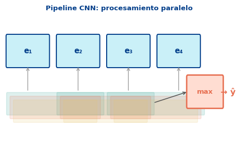
El Pipeline CNN

Texto → Embeddings → Conv1D → Pooling → Clasificador

Paso a paso: 1. Tokens → embeddings: matriz \(\mathbf{E} \in \mathbb{R}^{T \times d}\) 2. Filtros convolucionales en paralelo: \[h_i = \text{ReLU}(\mathbf{W} \cdot \mathbf{e}_{i:i+k-1} + b)\] 3. Global max pooling: \(\hat{h} = \max_i h_i\) 4. \(\hat{y} = \text{softmax}(\mathbf{W}\hat{\mathbf{h}} + \mathbf{b})\)

Note

Sin dependencia temporal: todos los \(h_i\) se calculan simultáneamente — el procesamiento es completamente paralelo.

Comparación Teórica

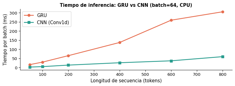
Eje 1: Paralelismo

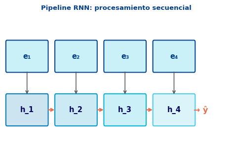
RNN — Secuencial por diseño

\[\mathbf{h}_t = f(\mathbf{h}_{t-1}, \mathbf{e}_t)\]

• Cada paso depende del anterior
• No se puede paralelizar a lo largo de \(T\)
• GPU infrautilizada para secuencias cortas
• Tiempo \(\propto T\) (longitud de la secuencia)

CNN — Paralelo por diseño

\[h_i = \text{ReLU}(\mathbf{W} \cdot \mathbf{e}_{i:i+k-1} + b)\]

• Todos los \(h_i\) son independientes entre sí
• Se calculan simultáneamente con nn.Conv1d
• GPU utilizada al máximo
• Tiempo \(\propto \log T\) en la práctica

Eje 2: Ventana de Contexto

RNN — Contexto global (en teoría)

• Accede a todo el pasado en \(\mathbf{h}_t\)
• En práctica: LSTM/GRU mitigan pero no eliminan el problema del gradiente
• Dependencias muy largas siguen siendo difíciles
• BiLSTM captura contexto en ambas direcciones

CNN — Contexto local (explícito)

• Cada filtro de tamaño \(k\) ve exactamente \(k\) tokens contiguos
• Campo receptivo de la capa \(l\): \(L(k-1)+1\)
• Para capturar dependencias largas: apilar capas o agrandar \(k\)
• Multi-tamaño: \(k \in \{3, 4, 5\}\) captura distintos n-gramas

	RNN/LSTM	CNN
Contexto teórico	Global (\(T\) tokens)	Local (\(k\) tokens por filtro)
Contexto práctico	~100–200 tokens útiles	Explícito, controlado por \(k\)
Dependencias largas	Con LSTM/GRU	Con capas apiladas
Captura de n-gramas	Implícita	Explícita y eficiente

Eje 3: Parámetros y Memoria

import torch.nn as nn

def count_params(model):
    return sum(p.numel() for p in model.parameters() if p.requires_grad)

V, D = 20000, 128   # vocabulario, dimensión embedding
H = 256             # tamaño oculto / canales

# GRU
gru_model = nn.Sequential(
    nn.Embedding(V, D),
    nn.GRU(D, H, batch_first=True)
)

# BiLSTM
class BiLSTM(nn.Module):
    def __init__(self):
        super().__init__()
        self.emb = nn.Embedding(V, D)
        self.lstm = nn.LSTM(D, H // 2, bidirectional=True, batch_first=True)
        self.fc = nn.Linear(H, 2)
    def forward(self, x):
        o, _ = self.lstm(self.emb(x))
        return self.fc(o[:, -1])

# TextCNN (Kim 2014)
class TextCNN(nn.Module):
    def __init__(self, filter_sizes=(3,4,5), num_filters=100):
        super().__init__()
        self.emb = nn.Embedding(V, D)
        self.convs = nn.ModuleList([
            nn.Conv1d(D, num_filters, fs) for fs in filter_sizes
        ])
        self.fc = nn.Linear(num_filters * len(filter_sizes), 2)
    def forward(self, x):
        e = self.emb(x).transpose(1, 2)
        pooled = [f.relu(conv(e)).max(dim=2).values for conv in self.convs]
        return self.fc(torch.cat(pooled, dim=1))

import torch.nn.functional as f
import torch

gru = nn.GRU(D, H, batch_first=True)
bilstm = BiLSTM()
textcnn = TextCNN()

print(f"GRU  (enc + emb):   {count_params(gru) + V*D:>10,} parámetros")
print(f"BiLSTM (full):      {count_params(bilstm):>10,} parámetros")
print(f"TextCNN (Kim 2014): {count_params(textcnn):>10,} parámetros")

GRU  (enc + emb):    2,856,448 parámetros
BiLSTM (full):       2,824,706 parámetros
TextCNN (Kim 2014):  2,714,502 parámetros

Tip

TextCNN es el modelo más ligero de los tres — una ventaja significativa cuando los recursos son limitados o se necesita inferencia rápida.

Benchmark Experimental

Configuración del Experimento

Dataset sintético de análisis de sentimiento

• 2 clases: positivo / negativo
• 4,000 ejemplos de entrenamiento, 1,000 de prueba
• Vocabulario de 5,000 tokens
• Longitudes de oración: 15–50 tokens
• Señal real basada en patrones de n-gramas

import torch
import torch.nn as nn
import numpy as np
from torch.utils.data import DataLoader, TensorDataset

torch.manual_seed(0)
np.random.seed(0)

VOCAB  = 5000
D      = 64
MAX_LEN = 40
N_TRAIN = 4000
N_TEST  = 1000

# Tokens con señal semántica
POS_TOKENS = list(range(10, 60))    # palabras positivas
NEG_TOKENS = list(range(60, 110))   # palabras negativas

def make_dataset(n, max_len=MAX_LEN):
    seqs, labels = [], []
    for _ in range(n):
        label = np.random.randint(0, 2)
        length = np.random.randint(15, max_len + 1)
        seq = np.random.randint(200, VOCAB, size=length)
        # insertar bigramas semánticos
        signal = POS_TOKENS if label == 1 else NEG_TOKENS
        for _ in range(np.random.randint(2, 5)):
            pos = np.random.randint(0, max(1, length - 2))
            seq[pos] = np.random.choice(signal)
            seq[pos + 1] = np.random.choice(signal)
        padded = np.zeros(max_len, dtype=np.int64)
        padded[:length] = seq[:max_len]
        seqs.append(padded)
        labels.append(label)
    return torch.tensor(seqs), torch.tensor(labels)

X_tr, y_tr = make_dataset(N_TRAIN)
X_te, y_te = make_dataset(N_TEST)
train_dl = DataLoader(TensorDataset(X_tr, y_tr), batch_size=64, shuffle=True)
test_dl  = DataLoader(TensorDataset(X_te, y_te), batch_size=256)
print(f"Train: {X_tr.shape}, Test: {X_te.shape}")

Train: torch.Size([4000, 40]), Test: torch.Size([1000, 40])

¿Por qué sintético?

• Control total sobre la señal
• Resultados reproducibles
• Permite aislar las diferencias arquitectónicas
• Dataset real → mismas tendencias, más ruido

Modelos a comparar:

Modelo	Tipo	Config
GRU	RNN	H=128
BiLSTM	RNN	H=64×2
TextCNN	CNN	k=3,4,5

Definición de los Tres Modelos

class GRUClassifier(nn.Module):
    def __init__(self, vocab=VOCAB, d=D, h=128):
        super().__init__()
        self.emb  = nn.Embedding(vocab, d, padding_idx=0)
        self.gru  = nn.GRU(d, h, batch_first=True)
        self.drop = nn.Dropout(0.3)
        self.fc   = nn.Linear(h, 2)

    def forward(self, x):
        e = self.drop(self.emb(x))
        _, h = self.gru(e)
        return self.fc(self.drop(h.squeeze(0)))


class BiLSTMClassifier(nn.Module):
    def __init__(self, vocab=VOCAB, d=D, h=64):
        super().__init__()
        self.emb  = nn.Embedding(vocab, d, padding_idx=0)
        self.lstm = nn.LSTM(d, h, bidirectional=True, batch_first=True)
        self.drop = nn.Dropout(0.3)
        self.fc   = nn.Linear(h * 2, 2)

    def forward(self, x):
        e = self.drop(self.emb(x))
        out, _ = self.lstm(e)
        # combinar últimos estados de ambas direcciones
        return self.fc(self.drop(out[:, -1]))


class TextCNNClassifier(nn.Module):
    def __init__(self, vocab=VOCAB, d=D, n_filters=64, filter_sizes=(3, 4, 5)):
        super().__init__()
        self.emb   = nn.Embedding(vocab, d, padding_idx=0)
        self.convs = nn.ModuleList([
            nn.Conv1d(d, n_filters, fs) for fs in filter_sizes
        ])
        self.drop  = nn.Dropout(0.3)
        self.fc    = nn.Linear(n_filters * len(filter_sizes), 2)

    def forward(self, x):
        e = self.emb(x).transpose(1, 2)      # (B, D, T)
        pooled = [
            torch.relu(conv(e)).max(dim=2).values
            for conv in self.convs
        ]
        return self.fc(self.drop(torch.cat(pooled, dim=1)))


models = {
    "GRU":     GRUClassifier(),
    "BiLSTM":  BiLSTMClassifier(),
    "TextCNN": TextCNNClassifier(),
}
for name, m in models.items():
    npar = sum(p.numel() for p in m.parameters() if p.requires_grad)
    print(f"{name:10s}: {npar:8,} parámetros")

GRU       :  394,754 parámetros
BiLSTM    :  386,818 parámetros
TextCNN   :  369,730 parámetros

Entrenamiento y Evaluación

import time

def train_model(model, train_dl, test_dl, epochs=10, lr=1e-3):
    opt = torch.optim.Adam(model.parameters(), lr=lr)
    criterion = nn.CrossEntropyLoss()
    history = {'train_acc': [], 'test_acc': []}

    t_start = time.perf_counter()
    for epoch in range(epochs):
        model.train()
        correct = total = 0
        for xb, yb in train_dl:
            opt.zero_grad()
            logits = model(xb)
            loss = criterion(logits, yb)
            loss.backward()
            opt.step()
            correct += (logits.argmax(1) == yb).sum().item()
            total   += len(yb)
        train_acc = correct / total

        model.eval()
        correct = total = 0
        with torch.no_grad():
            for xb, yb in test_dl:
                logits = model(xb)
                correct += (logits.argmax(1) == yb).sum().item()
                total   += len(yb)
        test_acc = correct / total
        history['train_acc'].append(train_acc)
        history['test_acc'].append(test_acc)

    elapsed = time.perf_counter() - t_start
    return history, elapsed

results = {}
print(f"{'Modelo':<12} {'Acc Train':>10} {'Acc Test':>10} {'Tiempo (s)':>12}")
print("-" * 48)
for name, model in models.items():
    hist, elapsed = train_model(model, train_dl, test_dl, epochs=10)
    results[name] = {'history': hist, 'time': elapsed}
    print(f"{name:<12} {hist['train_acc'][-1]:>10.3f} {hist['test_acc'][-1]:>10.3f} {elapsed:>12.2f}")

Modelo        Acc Train   Acc Test   Tiempo (s)
------------------------------------------------
GRU               0.992      0.997        21.81
BiLSTM            0.974      0.969        13.56
TextCNN           1.000      0.997         6.47

Curvas de Aprendizaje

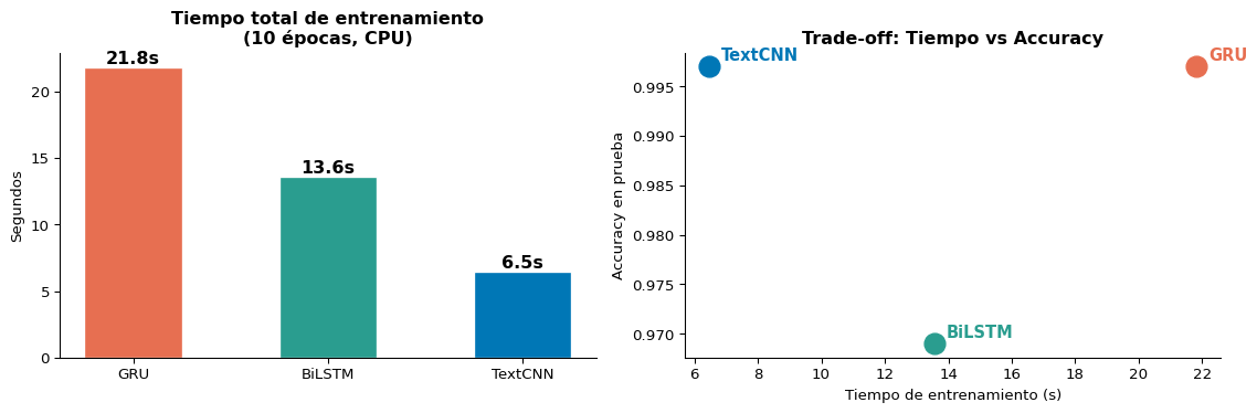
Comparación de Tiempos de Entrenamiento

Important

Observación clave: TextCNN alcanza accuracy competitivo en significativamente menos tiempo. La diferencia de velocidad se amplifica con GPUs y secuencias más largas.

Cuándo Usar Cada Uno

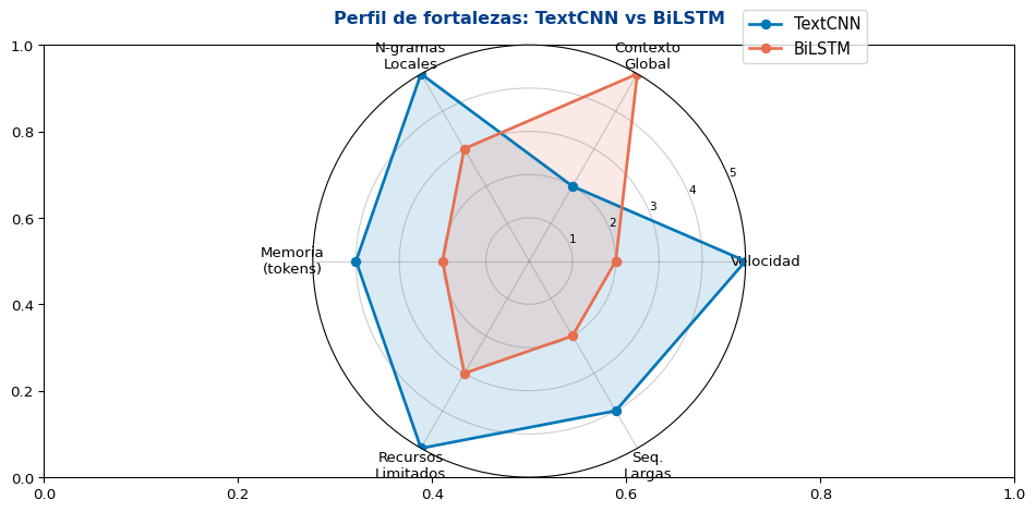
Guía de Decisión Práctica

Resumen Visual

Arquitecturas Híbridas

CNN + RNN: Lo Mejor de Ambos

Motivación

• CNN: extrae características locales eficientemente
• RNN: modela relaciones entre esas características

Pipeline

Texto → Embeddings
          ↓
       Conv1D  (captura n-gramas)
          ↓
       ReLU + pooling local
          ↓
       GRU/LSTM  (captura secuencia de patrones)
          ↓
       h_T → Clasificador

Tip

La CNN actúa como un extractor de características que reduce la longitud de secuencia antes de la RNN — reduciendo el problema del gradiente que desaparece.

class CNNRNNClassifier(nn.Module):
    """
    CNN extrae características locales,
    RNN captura su secuencia temporal.
    """
    def __init__(self, vocab=VOCAB, d=D,
                 n_filters=64, kernel=3, h=128):
        super().__init__()
        self.emb  = nn.Embedding(vocab, d, padding_idx=0)
        self.conv = nn.Conv1d(d, n_filters, kernel,
                              padding=kernel // 2)
        self.gru  = nn.GRU(n_filters, h, batch_first=True)
        self.drop = nn.Dropout(0.3)
        self.fc   = nn.Linear(h, 2)

    def forward(self, x):
        # CNN: extraer patrones locales
        e = self.emb(x).transpose(1, 2)    # (B,D,T)
        c = torch.relu(self.conv(e))        # (B,F,T)
        c = c.transpose(1, 2)              # (B,T,F)

        # RNN: modelar secuencia de patrones
        _, h = self.gru(self.drop(c))
        return self.fc(self.drop(h.squeeze(0)))


hybrid = CNNRNNClassifier()
npar = sum(p.numel() for p in hybrid.parameters() if p.requires_grad)
print(f"CNN+RNN: {npar:,} parámetros")

CNN+RNN: 407,106 parámetros

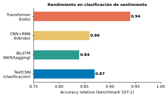
Benchmark Extendido: Incluyendo CNN+RNN

Resumen final:
Modelo         Acc Test   Tiempo (s)
------------------------------------
GRU               0.997        21.81
BiLSTM            0.969        13.56
TextCNN           0.997         6.47
CNN+RNN           0.986        21.90

Reflexión: ¿Cuál Es el Mejor Modelo?

No hay respuesta universal

“All models are wrong, but some are useful.”
— George Box

La elección depende de:

• Tarea: clasificación vs. generación vs. etiquetado
• Datos: longitud de secuencias, tamaño del dataset
• Recursos: GPU disponible, latencia requerida
• Baseline razonable: TextCNN es a menudo el mejor punto de partida por su velocidad

El panorama hoy (2024)

Important

Los Transformers (próxima semana) superan a CNN y RNN, pero requieren más datos y recursos.

Resumen y Cierre

Lo Que Aprendimos Hoy

Comparación teórica

Dimensión	CNN	RNN
Paralelismo	✅ Total	⚠️ Secuencial
N-gramas	✅ Explícito	⚠️ Implícito
Contexto largo	⚠️ Capas	✅ LSTM/GRU
Velocidad	✅ Rápido	⚠️ Lento
Parámetros	✅ Pocos	⚠️ Más

Resultado experimental

• En clasificación de texto: TextCNN ≈ BiLSTM en accuracy
• TextCNN: 2–3x más rápido en entrenamiento
• CNN+RNN: balance interesante para datos complejos

Cuándo usar cada uno

CNN: - Clasificación de texto / sentimiento - Detección de spam, tópicos - Recursos limitados - Baseline rápido

RNN/LSTM: - Traducción / generación - NER, POS tagging - Dependencias de largo alcance

CNN+RNN: - Documentos largos con estructura local - Cuando CNN sola no capta suficiente contexto

Para la Próxima Semana

Semana 9: Auto-Atención y Transformers

Note

Pregunta motivadora: ¿Puede un modelo capturar contexto global sin procesar la secuencia paso a paso (RNN) ni limitarse a ventanas locales (CNN)?

Respuesta: el mecanismo de auto-atención

\[\text{Attention}(Q, K, V) = \text{softmax}\!\left(\frac{QK^\top}{\sqrt{d_k}}\right)V\]

• Cada token puede “atender” a cualquier otro token directamente
• Sin dependencias secuenciales → completamente paralelo
• Complejidad: \(O(T^2)\) pero con GPU modernas es muy eficiente
• Base de BERT, GPT, y todos los LLMs modernos

Lecturas recomendadas

• Vaswani et al. (2017). Attention is All You Need
• Yin et al. (2017). Comparative Study of CNNs and RNNs for NLP
• Kim (2014). Convolutional Neural Networks for Sentence Classification

Para reflexionar

¿Por qué la atención supera tanto a CNN como a RNN en tareas de lenguaje si la primera se “ve” como más sencilla en su definición?

Referencias

• Kim, Y. (2014). Convolutional Neural Networks for Sentence Classification. EMNLP 2014.
• Yin, W., Kann, K., Yu, M., & Schütze, H. (2017). Comparative Study of CNN and RNN for Natural Language Processing. arXiv:1702.01923.
• Conneau, A., Schwenk, H., Barrault, L., & LeCun, Y. (2017). Very Deep Convolutional Networks for Text Classification. EACL 2017.
• Vaswani, A. et al. (2017). Attention Is All You Need. NeurIPS 2017.
• Zhou, C. et al. (2015). A C-LSTM Neural Network for Text Classification. arXiv:1511.08630.

¿Preguntas? 🙋

¡Gracias!

📧 fsuarez@ucb.edu.bo

🔗 Materiales: github.com/fjsuarez/ucb-nlp