Redes Neuronales Convolucionales para NLP

S2: Max Pooling Global vs. Local

Prof. Francisco Suárez

Universidad Católica Boliviana

2026-04-08

Agenda de Hoy

🔁 Repaso: Conv1D y el problema de longitud
🏊 Global Max Pooling: la estrategia dominante
📊 Average Pooling: la alternativa suave
🏆 K-Max Pooling: retener los top-\(k\)
🧪 Comparación experimental
⚙️ Pooling adaptativo para secuencias variables

Objetivo

Comparar diferentes estrategias de pooling para agregar información de secuencias de longitud variable en un vector de tamaño fijo, y entender cuándo usar cada una.

Prerequisitos: Conv1D para texto (S1)

El Problema de la Longitud Variable

Repaso: ¿Dónde Estamos?

Pipeline CNN para texto

Tokens → Embeddings (\(T \times d\))
Conv1D → Feature maps (\(T - k + 1\) valores por filtro)
??? Pooling ??? → Vector de tamaño fijo
Linear → Clasificación

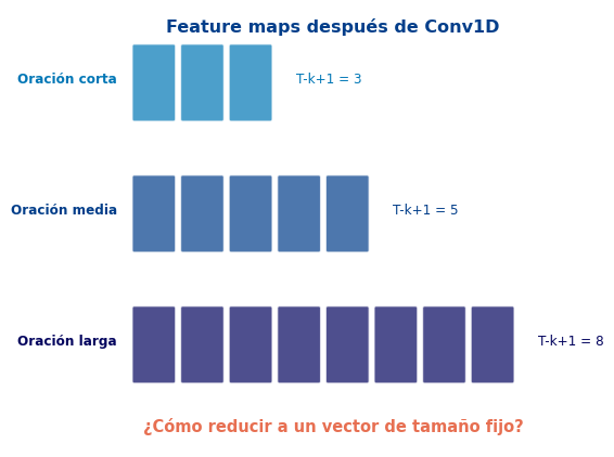
El problema

Las oraciones tienen longitud diferente:

“Great!” → \(T = 1\)
“The movie was absolutely fantastic” → \(T = 5\)
Después de Conv1D(\(k=3\)): salida de \(T-2\) valores
Necesitamos un vector de tamaño fijo para el clasificador

Global Max Pooling 🏊

La Estrategia Más Popular

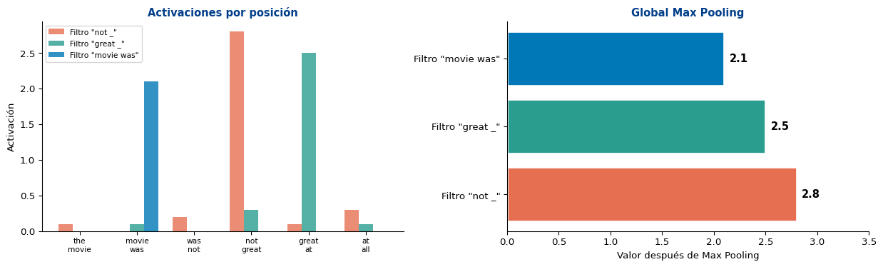
De cada feature map (lista de activaciones), tomar el valor máximo:

\[\hat{h}_j = \max_{i=1}^{T-k+1} h_j^{(i)}\]

Intuición

Cada filtro detecta un patrón (n-grama)
Max pooling pregunta: “¿Este patrón aparece en algún lugar de la oración?”
No importa dónde aparece
Invariante a la posición

Propiedades

Entrada: \((N_{\text{filtros}}, T-k+1)\)
Salida: \((N_{\text{filtros}},)\) — un escalar por filtro
Siempre produce vector de tamaño fijo
Pierde información posicional

Code

import torch
import torch.nn as nn

# Simular feature maps de un filtro para 3 oraciones de diferente longitud
torch.manual_seed(42)

maps = {
    "short  (T=5)":  torch.relu(torch.randn(1, 4, 3)),   # 4 filtros, 3 posiciones
    "medium (T=8)":  torch.relu(torch.randn(1, 4, 6)),   # 4 filtros, 6 posiciones
    "long   (T=15)": torch.relu(torch.randn(1, 4, 13)),  # 4 filtros, 13 posiciones
}

print("Global Max Pooling: extrae 1 valor (máximo) por filtro")
print("=" * 55)
for name, fmap in maps.items():
    pooled = fmap.max(dim=2).values  # (1, 4)
    print(f"  {name}:  feature map {list(fmap.shape)} → max pooled {list(pooled.shape)}")

Global Max Pooling: extrae 1 valor (máximo) por filtro
=======================================================
  short  (T=5):  feature map [1, 4, 3] → max pooled [1, 4]
  medium (T=8):  feature map [1, 4, 6] → max pooled [1, 4]
  long   (T=15):  feature map [1, 4, 13] → max pooled [1, 4]

Visualización: ¿Qué Captura Max Pooling?

Lo que se pierde

Max pooling solo retiene la activación más fuerte. Si un patrón aparece 3 veces o 30 veces, el resultado es el mismo. Perdemos información sobre frecuencia y posición.

Average Pooling 📊

La Alternativa Suave

En lugar del máximo, tomar el promedio de las activaciones:

\[\hat{h}_j = \frac{1}{T-k+1} \sum_{i=1}^{T-k+1} h_j^{(i)}\]

Ventajas

Captura frecuencia: si un patrón aparece muchas veces, el promedio es alto
Más suave que max: menos sensible a outliers
Funciona bien cuando el tono general importa

Desventajas

Diluye señales fuertes pero poco frecuentes
Una negación en una oración larga puede perderse
No captura “al menos una vez” como max pooling

Code

# Comparar max vs average pooling
feature_map = torch.tensor([[[0.1, 0.0, 3.5, 0.2, 0.1]]])  # (1, 1, 5)

max_pool = feature_map.max(dim=2).values
avg_pool = feature_map.mean(dim=2)

print("Feature map:", feature_map.squeeze().tolist())
print(f"Max pooling: {max_pool.item():.2f}  ← captura el pico")
print(f"Avg pooling: {avg_pool.item():.2f}  ← diluye el pico")

# Caso: patrón frecuente
feature_map2 = torch.tensor([[[1.2, 1.5, 1.3, 1.4, 1.1]]])
max_pool2 = feature_map2.max(dim=2).values
avg_pool2 = feature_map2.mean(dim=2)

print(f"\nFeature map: {feature_map2.squeeze().tolist()}")
print(f"Max pooling: {max_pool2.item():.2f}  ← similar al promedio")
print(f"Avg pooling: {avg_pool2.item():.2f}  ← captura la consistencia")

Feature map: [0.10000000149011612, 0.0, 3.5, 0.20000000298023224, 0.10000000149011612]
Max pooling: 3.50  ← captura el pico
Avg pooling: 0.78  ← diluye el pico

Feature map: [1.2000000476837158, 1.5, 1.2999999523162842, 1.399999976158142, 1.100000023841858]
Max pooling: 1.50  ← similar al promedio
Avg pooling: 1.30  ← captura la consistencia

Ejemplo: ¿Cuándo Importa la Diferencia?

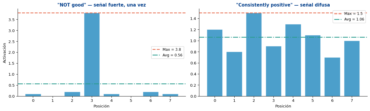
La clave

Max pooling es mejor para patrones específicos y puntuales (negación, palabras clave)
Avg pooling es mejor para tono general (un texto consistentemente positivo)
En la práctica, max pooling domina para clasificación de texto (Kim, 2014)

K-Max Pooling 🏆

Retener los Top-\(k\) Valores

Propuesto por Kalchbrenner et al. (2014): en lugar de 1 solo valor, retener los \(k\) valores más altos (preservando su orden):

\[\text{k-max}(\mathbf{h}) = \text{sort}(\text{top-}k(\mathbf{h}))\]

Ventajas

Retiene múltiples señales relevantes
Preserva el orden relativo de los top-\(k\) valores
Más información que max pooling
\(k=1\) es equivalente a global max pooling

Desventajas

Introduce hiperparámetro \(k\)
Vector de salida es de tamaño \(k \times N_{\text{filtros}}\)
Puede ser excesivo para textos cortos

Code

def k_max_pooling(x, k):
    """
    x: (batch, channels, length)
    Retorna: (batch, channels, k) — top-k valores en orden original
    """
    topk_vals, topk_idx = x.topk(k, dim=2)
    # Ordenar por posición para preservar el orden de la secuencia
    sorted_idx = topk_idx.sort(dim=2).values
    return x.gather(2, sorted_idx)

# Ejemplo
feature_map = torch.tensor([[[0.1, 2.5, 0.3, 3.1, 0.8, 1.9, 0.2]]])
print(f"Feature map:   {feature_map.squeeze().tolist()}")
print(f"Max pooling:   {feature_map.max(dim=2).values.squeeze().tolist()}")
print(f"K-max (k=3):   {k_max_pooling(feature_map, k=3).squeeze().tolist()}")
print(f"Avg pooling:   {feature_map.mean(dim=2).squeeze().item():.2f}")

Feature map:   [0.10000000149011612, 2.5, 0.30000001192092896, 3.0999999046325684, 0.800000011920929, 1.899999976158142, 0.20000000298023224]
Max pooling:   3.0999999046325684
K-max (k=3):   [2.5, 3.0999999046325684, 1.899999976158142]
Avg pooling:   1.27

Comparación Visual de las 3 Estrategias

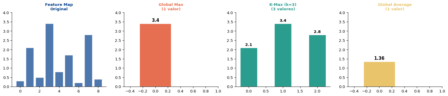
Estrategia	Salida por filtro	Información retenida	Mejor para
Global Max	1 escalar	Solo el pico	Patrones puntuales
Global Average	1 escalar	Promedio general	Tono difuso
K-Max	\(k\) escalares	Top-\(k\) en orden	Balance de ambos

Comparación Experimental 🧪

Clasificador CNN con Diferentes Poolings

Code

import random
import torch.optim as optim

torch.manual_seed(42)
random.seed(42)
np.random.seed(42)

# --- Datos: sentimiento sintético (reusar vocabulario simple) ---
positive_words = ["great", "amazing", "wonderful", "excellent", "fantastic", "brilliant",
                  "superb", "loved", "enjoyed", "outstanding", "perfect", "best"]
negative_words = ["terrible", "horrible", "awful", "worst", "dreadful", "boring",
                  "bad", "hated", "poor", "disappointing", "weak", "disaster"]
neutral_words = ["the", "a", "movie", "film", "was", "is", "this", "that", "very",
                 "really", "quite", "it", "and", "but", "with", "not"]

all_words = sorted(set(positive_words + negative_words + neutral_words))
word2idx = {"<PAD>": 0}
for w in all_words:
    word2idx[w] = len(word2idx)
VOCAB = len(word2idx)

def make_sentence(label, min_len=5, max_len=12):
    length = random.randint(min_len, max_len)
    words_pool = positive_words if label == 1 else negative_words
    n_key = random.randint(1, 3)
    sent = random.choices(neutral_words, k=length - n_key) + random.choices(words_pool, k=n_key)
    random.shuffle(sent)
    return sent

def encode(sent, max_len=12):
    ids = [word2idx.get(w, 0) for w in sent[:max_len]]
    return ids + [0] * (max_len - len(ids))

# Generar
data = []
for _ in range(800):
    data.append((make_sentence(1), 1))
    data.append((make_sentence(0), 0))
random.shuffle(data)

X = torch.tensor([encode(s) for s, _ in data])
y = torch.tensor([l for _, l in data])
split = int(0.8 * len(X))
X_train, y_train = X[:split], y[:split]
X_test, y_test = X[split:], y[split:]
print(f"Vocab: {VOCAB} | Train: {len(X_train)} | Test: {len(X_test)}")

Vocab: 41 | Train: 1280 | Test: 320

Code

class CNNWithPooling(nn.Module):
    def __init__(self, vocab_size, embed_dim, n_filters, kernel_sizes,
                 n_classes, pooling='max', k_max=3, pad_idx=0):
        super().__init__()
        self.pooling = pooling
        self.k_max_val = k_max
        self.embedding = nn.Embedding(vocab_size, embed_dim, padding_idx=pad_idx)
        self.convs = nn.ModuleList([
            nn.Conv1d(embed_dim, n_filters, k) for k in kernel_sizes
        ])
        
        if pooling == 'kmax':
            fc_input = n_filters * len(kernel_sizes) * k_max
        else:
            fc_input = n_filters * len(kernel_sizes)
        
        self.dropout = nn.Dropout(0.3)
        self.fc = nn.Linear(fc_input, n_classes)
    
    def forward(self, x):
        emb = self.embedding(x).permute(0, 2, 1)
        
        conv_outs = []
        for conv in self.convs:
            h = torch.relu(conv(emb))
            if self.pooling == 'max':
                h = h.max(dim=2).values
            elif self.pooling == 'avg':
                h = h.mean(dim=2)
            elif self.pooling == 'kmax':
                k = min(self.k_max_val, h.size(2))
                h = h.topk(k, dim=2).values
                h = h.view(h.size(0), -1)
            conv_outs.append(h)
        
        cat = torch.cat(conv_outs, dim=1)
        return self.fc(self.dropout(cat))

# Entrenar las 3 variantes
def train_eval(pooling, k_max=3, n_epochs=40):
    model = CNNWithPooling(VOCAB, embed_dim=32, n_filters=32, kernel_sizes=[2,3,4],
                            n_classes=2, pooling=pooling, k_max=k_max)
    opt = optim.Adam(model.parameters(), lr=0.003)
    crit = nn.CrossEntropyLoss()
    losses = []
    for epoch in range(n_epochs):
        model.train()
        idx = torch.randperm(len(X_train))
        e_loss, n_b = 0, 0
        for i in range(0, len(X_train), 64):
            bi = idx[i:i+64]
            loss = crit(model(X_train[bi]), y_train[bi])
            opt.zero_grad(); loss.backward(); opt.step()
            e_loss += loss.item(); n_b += 1
        losses.append(e_loss / n_b)
    model.eval()
    with torch.no_grad():
        acc = (model(X_test).argmax(1) == y_test).float().mean().item()
    n_params = sum(p.numel() for p in model.parameters())
    return losses, acc, n_params

results = {}
for pool in ['max', 'avg', 'kmax']:
    losses, acc, n_params = train_eval(pool)
    results[pool] = {'losses': losses, 'acc': acc, 'params': n_params}
    label = f"{'K-Max (k=3)' if pool == 'kmax' else pool.capitalize()}"
    print(f"{label:>12s}:  Acc = {acc:.1%}  |  Params = {n_params:,}")

         Max:  Acc = 99.7%  |  Params = 10,818
         Avg:  Acc = 99.7%  |  Params = 10,818
 K-Max (k=3):  Acc = 99.7%  |  Params = 11,202

Resultados: Curvas y Accuracy

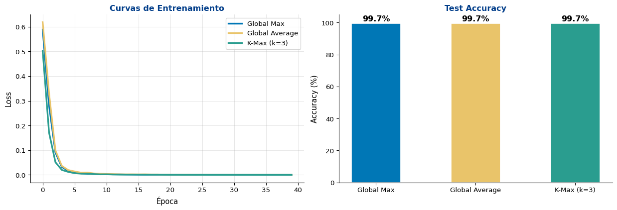
Tabla Resumen

| Pooling | Accuracy | Parámetros | Salida por filtro |
|:--------|:---------|:-----------|:------------------|
| **Global Max** | 99.7% | 10,818 | 1 escalar |
| **Global Average** | 99.7% | 10,818 | 1 escalar |
| **K-Max (k=3)** | 99.7% | 11,202 | 3 escalares |

Observaciones

Max pooling suele ganar en tareas donde hay palabras clave discriminativas (sentimiento)
Average pooling puede ser mejor en tareas donde el tono general importa (detección de tópicos)
K-max pooling ofrece más información pero con más parámetros en la capa Linear
En la literatura, max pooling es la opción por defecto para CNNs de texto

Pooling para Secuencias Variables ⚙️

Padding y su Efecto en Pooling

El problema del padding

Cuando hay tokens <PAD>, las activaciones convolucionales sobre padding deberían ser cero o cercanas a cero.

Max pooling: no se ve afectado (ignora valores bajos/cero)
Average pooling: ¡sí se ve afectado! Los ceros diluyen el promedio

Solución: Average pooling adaptativo

Dividir solo por la longitud real, no la longitud con padding:

\[\hat{h}_j = \frac{1}{L_{\text{real}}} \sum_{i=1}^{L_{\text{real}}} h_j^{(i)}\]

Code

# Demostrar el efecto del padding en average pooling
activations_real = torch.tensor([[[2.1, 1.5, 1.8, 0.0, 0.0]]])  # 3 reales + 2 PAD

# Average naive (incluye padding)
avg_naive = activations_real.mean(dim=2)

# Average adaptativo (solo cuenta tokens reales)
real_length = 3
avg_adaptive = activations_real[:, :, :real_length].mean(dim=2)

max_pool = activations_real.max(dim=2).values

print(f"Activaciones:     {activations_real.squeeze().tolist()}")
print(f"  (3 reales + 2 PAD)")
print(f"\nMax pooling:      {max_pool.item():.2f}  ← no afectado por PAD")
print(f"Avg naive:        {avg_naive.item():.2f}  ← diluido por PAD (÷5)")
print(f"Avg adaptativo:   {avg_adaptive.item():.2f}  ← correcto (÷3)")

Activaciones:     [2.0999999046325684, 1.5, 1.7999999523162842, 0.0, 0.0]
  (3 reales + 2 PAD)

Max pooling:      2.10  ← no afectado por PAD
Avg naive:        1.08  ← diluido por PAD (÷5)
Avg adaptativo:   1.80  ← correcto (÷3)

`AdaptiveMaxPool1d` en PyTorch

PyTorch ofrece capas adaptativas que producen un tamaño fijo sin importar la entrada:

Code

# AdaptiveMaxPool1d: salida de tamaño fijo independiente de la entrada
pool_1 = nn.AdaptiveMaxPool1d(output_size=1)   # Global max pooling
pool_3 = nn.AdaptiveMaxPool1d(output_size=3)   # K-max-like (k=3)

# Secuencias de diferente longitud
short = torch.relu(torch.randn(1, 4, 5))   # 4 filtros, 5 posiciones
long = torch.relu(torch.randn(1, 4, 20))   # 4 filtros, 20 posiciones

print("AdaptiveMaxPool1d(output_size=1):")
print(f"  Input (1,4,5)  → Output {pool_1(short).shape}")
print(f"  Input (1,4,20) → Output {pool_1(long).shape}")
print(f"\nAdaptiveMaxPool1d(output_size=3):")
print(f"  Input (1,4,5)  → Output {pool_3(short).shape}")
print(f"  Input (1,4,20) → Output {pool_3(long).shape}")

AdaptiveMaxPool1d(output_size=1):
  Input (1,4,5)  → Output torch.Size([1, 4, 1])
  Input (1,4,20) → Output torch.Size([1, 4, 1])

AdaptiveMaxPool1d(output_size=3):
  Input (1,4,5)  → Output torch.Size([1, 4, 3])
  Input (1,4,20) → Output torch.Size([1, 4, 3])

En la práctica

nn.AdaptiveMaxPool1d(1) es equivalente a global max pooling y es la forma “limpia” de implementarlo en PyTorch. Es independiente de la longitud de la secuencia.

Resumen

Lo Que Aprendimos Hoy

Estrategias de Pooling

Tipo	Captura
Max	¿Aparece el patrón? (binario)
Average	¿Cuánto aparece en promedio?
K-Max	¿Cuáles son las top-\(k\) activaciones?

Max pooling es el estándar para clasificación de texto
Average pooling sufre con padding → usar versión adaptativa
K-max pooling ofrece más información, pero con más parámetros

Práctica

Tensor.max(dim=2) — global max pooling manual
nn.AdaptiveMaxPool1d(1) — versión PyTorch
Tensor.mean(dim=2) — average pooling (cuidado con padding)
Tensor.topk(k, dim=2) — k-max pooling
Combinar poolings → concatenar (max + avg)

Para la Próxima Sesión 📚

Semana 8, S3: Comparación RNNs vs. CNNs para Clasificación

Benchmark sistemático: GRU vs. LSTM vs. BiLSTM vs. CNN
¿Cuándo usar cada arquitectura?
Eficiencia computacional (tiempo, parámetros, memoria)
Modelos híbridos: CNN + RNN

Lectura:

Yin et al. (2017): Comparative Study of CNN and RNN for NLP
Conneau et al. (2017): Very Deep Convolutional Networks for Text Classification
Kim (2014): Convolutional Neural Networks for Sentence Classification

Recordatorio:

Quiz 6 cubre Seq2Seq y Atención (Semana 7) 🧮

¿Preguntas? 🙋

¡Gracias!

📧 fsuarez@ucb.edu.bo

🔗 Materiales: github.com/fjsuarez/ucb-nlp

Redes Neuronales Convolucionales para NLP

Agenda de Hoy

El Problema de la Longitud Variable

Repaso: ¿Dónde Estamos?

Pipeline CNN para texto

El problema

Global Max Pooling 🏊

La Estrategia Más Popular

Intuición

Propiedades

Visualización: ¿Qué Captura Max Pooling?

Average Pooling 📊

La Alternativa Suave

Ventajas

Desventajas

Ejemplo: ¿Cuándo Importa la Diferencia?

K-Max Pooling 🏆

Retener los Top-\(k\) Valores

Ventajas

Desventajas

Comparación Visual de las 3 Estrategias

Comparación Experimental 🧪

Clasificador CNN con Diferentes Poolings

Resultados: Curvas y Accuracy

Tabla Resumen

Pooling para Secuencias Variables ⚙️

Padding y su Efecto en Pooling

El problema del padding

Solución: Average pooling adaptativo

AdaptiveMaxPool1d en PyTorch

Resumen

Lo Que Aprendimos Hoy

Estrategias de Pooling

Práctica

Para la Próxima Sesión 📚

¿Preguntas? 🙋

`AdaptiveMaxPool1d` en PyTorch