Secuencia a Secuencia (Seq2Seq)
S3: El Mecanismo de Atención
Prof. Francisco Suárez
Universidad Católica Boliviana
2026-03-31
Agenda de Hoy
- 🔍 Repaso: el cuello de botella
- 💡 Intuición de la Atención
- 📐 Atención de Bahdanau (aditiva)
- ⚡ Atención de Luong (multiplicativa)
- 🧪 Experimento: Seq2Seq con atención
- 🗺️ Mapas de atención y visualización
Objetivo
Entender el mecanismo de Atención que permite al decoder consultar selectivamente diferentes partes de la entrada, resolviendo el cuello de botella del vector de contexto fijo.
Prerequisitos: Seq2Seq, NMT (Semana 7 S1-S2)
El Cuello de Botella (Repaso)
El Problema que Resolvemos Hoy
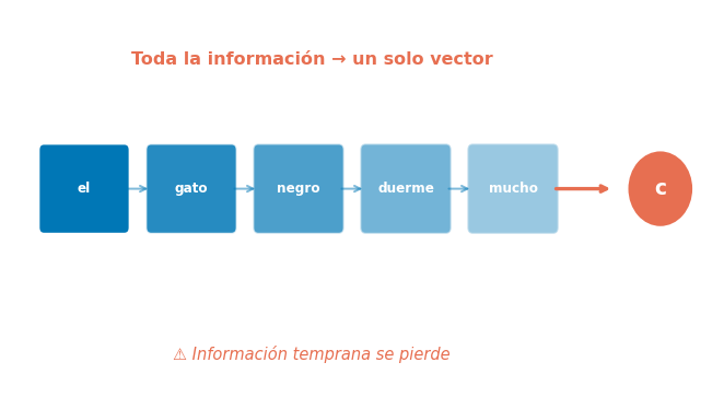
Seq2Seq sin atención
El encoder comprime toda la secuencia en un solo vector:
\[x_1, x_2, \ldots, x_{T_x} \rightarrow \mathbf{c} \in \mathbb{R}^{D_h}\]
El decoder solo ve \(\mathbf{c}\) → pierde detalles de la entrada.
Problemas observados:
- Rendimiento se degrada con secuencias largas
- El decoder no sabe dónde mirar en la entrada
- Información temprana se pierde por el vanishing gradient
Cho et al. (2014) confirmaron
El rendimiento de NMT cae dramáticamente en oraciones de más de ~20 tokens. El cuello de botella del vector fijo es la causa principal.
La Idea de la Atención 💡
Intuición: “Mirar Hacia Atrás”
En lugar de comprimir toda la entrada en un solo vector, ¿qué tal si el decoder pudiera consultar las representaciones de todos los tokens de entrada en cada paso?
Analogía humana
Cuando un traductor traduce una oración:
- No lee toda la oración, la memoriza, y luego traduce de memoria
- Consulta diferentes partes del texto original según la palabra que está traduciendo
- “el gato” → mira “the cat”
- “duerme” → mira “sleeps”
La solución
En cada paso de decodificación \(t\):
- Almacenar todos los estados del encoder: \(h_1, h_2, \ldots, h_{T_x}\)
- Calcular qué tan relevante es cada \(h_j\) para el paso actual
- Promediar ponderadamente estos estados → vector de contexto dinámico \(\mathbf{c}_t\)
\[\mathbf{c}_t = \sum_{j=1}^{T_x} \alpha_{t,j} \cdot h_j\]
Atención: Visión General
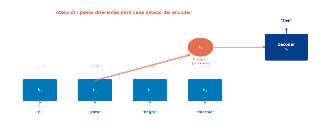
Diferencia clave con Seq2Seq estándar
El vector de contexto \(\mathbf{c}_t\) es diferente en cada paso de decodificación. Ya no es un vector fijo — es una combinación ponderada de los estados del encoder que cambia según lo que el decoder necesita.
Atención de Bahdanau (Aditiva) 📐
Bahdanau et al. (2015)
El paper fundacional: “Neural Machine Translation by Jointly Learning to Align and Translate”
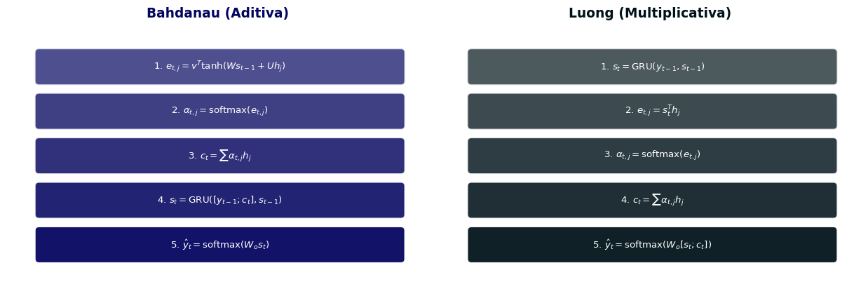
Paso a paso
1. Score de alineación — ¿qué tan relevante es \(h_j\) para el estado del decoder \(s_{t-1}\)?
\[e_{t,j} = v_a^\top \tanh(W_a \cdot s_{t-1} + U_a \cdot h_j)\]
2. Pesos de atención — normalizar con softmax:
\[\alpha_{t,j} = \frac{\exp(e_{t,j})}{\sum_{k=1}^{T_x} \exp(e_{t,k})}\]
3. Vector de contexto dinámico — combinar estados del encoder:
\[\mathbf{c}_t = \sum_{j=1}^{T_x} \alpha_{t,j} \cdot h_j\]
4. Actualizar el decoder — usando contexto + input:
\[s_t = \text{GRU}([\text{emb}(y_{t-1}); \mathbf{c}_t], \; s_{t-1})\]
¿Por qué “aditiva”?
Porque el score combina \(s_{t-1}\) y \(h_j\) con una suma seguida de \(\tanh\) y un vector aprendido \(v_a\). Los parámetros \(W_a\), \(U_a\) y \(v_a\) se aprenden durante entrenamiento.
Implementación: Atención de Bahdanau
Code
import torch
import torch.nn as nn
import torch.nn.functional as F

class BahdanauAttention(nn.Module):
    def __init__(self, hidden_dim):
        super().__init__()
        self.W_a = nn.Linear(hidden_dim, hidden_dim, bias=False)
        self.U_a = nn.Linear(hidden_dim, hidden_dim, bias=False)
        self.v_a = nn.Linear(hidden_dim, 1, bias=False)

    def forward(self, decoder_hidden, encoder_outputs):
        """
        decoder_hidden: (batch, hidden_dim) — s_{t-1}
        encoder_outputs: (batch, src_len, hidden_dim) — h_1, ..., h_{T_x}
        """
        # decoder_hidden → (batch, 1, hidden_dim) para broadcasting
        dec_expanded = decoder_hidden.unsqueeze(1)

        # Score: v^T tanh(W·s + U·h) → (batch, src_len, 1)
        energy = self.v_a(torch.tanh(
            self.W_a(dec_expanded) + self.U_a(encoder_outputs)
        ))

        # Pesos: softmax sobre src_len → (batch, src_len)
        attention_weights = F.softmax(energy.squeeze(-1), dim=-1)

        # Contexto: promedio ponderado → (batch, hidden_dim)
        context = torch.bmm(attention_weights.unsqueeze(1),
                           encoder_outputs).squeeze(1)

        return context, attention_weights

# Demo
torch.manual_seed(42)
attn = BahdanauAttention(hidden_dim=64)
fake_dec_h = torch.randn(4, 64)        # batch=4
fake_enc_out = torch.randn(4, 8, 64)   # src_len=8
ctx, weights = attn(fake_dec_h, fake_enc_out)
print(f"Contexto:  {ctx.shape}")          # (4, 64)
print(f"Pesos:     {weights.shape}")      # (4, 8)
print(f"Suma pesos: {weights[0].sum().item():.4f}")  # = 1.0
print(f"Pesos[0]:  {weights[0].data.numpy().round(3)}")
Contexto: torch.Size([4, 64])
Pesos: torch.Size([4, 8])
Suma pesos: 1.0000
Pesos[0]: [0.189 0.101 0.086 0.086 0.131 0.124 0.123 0.16 ]Atención de Luong (Multiplicativa) ⚡
Luong et al. (2015)
“Effective Approaches to Attention-based Neural Machine Translation” — versión más simple y eficiente.
Tres variantes de score
| Nombre | Score \(e_{t,j}\) |
|---|---|
| dot | \(s_t^\top h_j\) |
| general | \(s_t^\top W_a h_j\) |
| concat | \(v_a^\top \tanh(W_a [s_t; h_j])\) |
La variante dot es la más usada:
- No tiene parámetros aprendibles
- Extremadamente eficiente (solo producto punto)
- Funciona bien cuando \(s_t\) y \(h_j\) están en el mismo espacio
Diferencias con Bahdanau
| Aspecto | Bahdanau | Luong |
|---|---|---|
| Score | Aditivo (MLP) | Multiplicativo (dot) |
| Estado decoder | \(s_{t-1}\) | \(s_t\) (actual) |
| Contexto se usa en | Input del GRU | Output layer |
| Complejidad | \(O(D_h^2)\) | \(O(D_h)\) para dot |
En la práctica
La variante dot product de Luong evolucionó en el Scaled Dot-Product Attention del Transformer (Semana 9).
Implementación: Atención de Luong (dot)
Code
class LuongAttention(nn.Module):
    def __init__(self, hidden_dim, method='dot'):
        super().__init__()
        self.method = method
        if method == 'general':
            self.W_a = nn.Linear(hidden_dim, hidden_dim, bias=False)

    def forward(self, decoder_hidden, encoder_outputs):
        """
        decoder_hidden: (batch, hidden_dim) — s_t (estado actual)
        encoder_outputs: (batch, src_len, hidden_dim)
        """
        if self.method == 'dot':
            # Score: s_t^T · h_j → (batch, src_len)
            energy = torch.bmm(encoder_outputs,
                              decoder_hidden.unsqueeze(-1)).squeeze(-1)
        elif self.method == 'general':
            energy = torch.bmm(self.W_a(encoder_outputs),
                              decoder_hidden.unsqueeze(-1)).squeeze(-1)

        attention_weights = F.softmax(energy, dim=-1)
        context = torch.bmm(attention_weights.unsqueeze(1),
                           encoder_outputs).squeeze(1)

        return context, attention_weights

# Comparar ambas
luong_attn = LuongAttention(hidden_dim=64, method='dot')
ctx_l, weights_l = luong_attn(fake_dec_h, fake_enc_out)
print(f"Bahdanau pesos: {weights[0].data.numpy().round(3)}")
print(f"Luong    pesos: {weights_l[0].data.numpy().round(3)}")
print(f"\nBahdanau: {sum(p.numel() for p in attn.parameters()):,} parámetros")
print(f"Luong (dot): {sum(p.numel() for p in luong_attn.parameters()):,} parámetros")
Bahdanau pesos: [0.189 0.101 0.086 0.086 0.131 0.124 0.123 0.16 ]
Luong pesos: [0.022 0.964 0. 0. 0. 0.014 0. 0. ]
Bahdanau: 8,256 parámetros
Luong (dot): 0 parámetrosComparación Visual: Bahdanau vs. Luong
Observación clave
Bahdanau calcula la atención antes de actualizar el decoder (usa \(s_{t-1}\)). Luong calcula la atención después (usa \(s_t\)). En la práctica, ambas funcionan bien.
Experimento: Seq2Seq con Atención 🧪
Modelo Completo con Atención
Code
import random

class AttentionEncoder(nn.Module):
    def __init__(self, vocab_size, embed_dim, hidden_dim):
        super().__init__()
        self.embedding = nn.Embedding(vocab_size, embed_dim)
        self.rnn = nn.GRU(embed_dim, hidden_dim, batch_first=True)

    def forward(self, src):
        embedded = self.embedding(src)
        outputs, hidden = self.rnn(embedded)
        return outputs, hidden  # ← Ahora retornamos TODOS los estados

class AttentionDecoder(nn.Module):
    def __init__(self, vocab_size, embed_dim, hidden_dim):
        super().__init__()
        self.embedding = nn.Embedding(vocab_size, embed_dim)
        self.attention = BahdanauAttention(hidden_dim)
        self.rnn = nn.GRU(embed_dim + hidden_dim, hidden_dim, batch_first=True)
        self.fc_out = nn.Linear(hidden_dim * 2, vocab_size)

    def forward(self, input_token, hidden, encoder_outputs):
        embedded = self.embedding(input_token)          # (batch, 1, embed_dim)

        # Atención: contexto dinámico
        context, attn_weights = self.attention(
            hidden.squeeze(0), encoder_outputs           # s_{t-1}, h_1..h_T
        )

        # Concatenar embedding + contexto como input del GRU
        rnn_input = torch.cat([embedded, context.unsqueeze(1)], dim=-1)
        output, hidden = self.rnn(rnn_input, hidden)

        # Predicción: concatenar output + contexto
        prediction = self.fc_out(torch.cat([output.squeeze(1), context], dim=-1))

        return prediction, hidden, attn_weights
Entrenamiento: Inversión de Secuencias
Code
import torch.optim as optim

PAD, SOS, EOS = 0, 1, 2
NUM_DIGITS = 10
VOCAB_SIZE = NUM_DIGITS + 3

def generate_pairs(n, min_len=4, max_len=10):
    src_list, trg_list = [], []
    for _ in range(n):
        length = random.randint(min_len, max_len)
        seq = [random.randint(3, VOCAB_SIZE - 1) for _ in range(length)]
        src_list.append(seq + [PAD] * (max_len - length))
        trg_list.append(list(reversed(seq)) + [EOS] + [PAD] * (max_len - length))
    return torch.tensor(src_list), torch.tensor(trg_list)

torch.manual_seed(42)
random.seed(42)
train_src, train_trg = generate_pairs(3000)
test_src, test_trg = generate_pairs(300)

EMBED_DIM = 32
HIDDEN_DIM = 64
BATCH_SIZE = 128
N_EPOCHS = 40

enc_attn = AttentionEncoder(VOCAB_SIZE, EMBED_DIM, HIDDEN_DIM)
dec_attn = AttentionDecoder(VOCAB_SIZE, EMBED_DIM, HIDDEN_DIM)

params = list(enc_attn.parameters()) + list(dec_attn.parameters())
optimizer = optim.Adam(params, lr=0.003)
criterion = nn.CrossEntropyLoss(ignore_index=PAD)

losses_attn = []
for epoch in range(N_EPOCHS):
    enc_attn.train(); dec_attn.train()
    epoch_loss, n_b = 0, 0
    idx = torch.randperm(len(train_src))
    for i in range(0, len(train_src), BATCH_SIZE):
        bi = idx[i:i+BATCH_SIZE]
        src, trg = train_src[bi], train_trg[bi]

        enc_out, hidden = enc_attn(src)
        input_tok = torch.full((src.size(0), 1), SOS, dtype=torch.long)

        all_preds = []
        for t in range(trg.size(1)):
            pred, hidden, _ = dec_attn(input_tok, hidden, enc_out)
            all_preds.append(pred)
            if random.random() < max(0.1, 1 - epoch/N_EPOCHS):
                input_tok = trg[:, t:t+1]
            else:
                input_tok = pred.argmax(1, keepdim=True)

        outputs = torch.stack(all_preds, dim=1)
        loss = criterion(outputs.reshape(-1, VOCAB_SIZE), trg.reshape(-1))

        optimizer.zero_grad()
        loss.backward()
        torch.nn.utils.clip_grad_norm_(params, 1.0)
        optimizer.step()
        epoch_loss += loss.item()
        n_b += 1

    losses_attn.append(epoch_loss / n_b)
    if (epoch+1) % 10 == 0:
        print(f"Época {epoch+1:3d}/{N_EPOCHS} | Loss: {losses_attn[-1]:.4f}")
Época 10/40 | Loss: 0.0172
Época 20/40 | Loss: 0.0009
Época 30/40 | Loss: 0.0004
Época 40/40 | Loss: 0.0002Evaluación y Comparación
Code
# Evaluación con atención
enc_attn.eval(); dec_attn.eval()
all_preds_attn = []
all_weights = []

with torch.no_grad():
    enc_out, hidden = enc_attn(test_src)
    input_tok = torch.full((test_src.size(0), 1), SOS, dtype=torch.long)

    for t in range(test_trg.size(1)):
        pred, hidden, attn_w = dec_attn(input_tok, hidden, enc_out)
        all_preds_attn.append(pred.argmax(1))
        all_weights.append(attn_w)
        input_tok = pred.argmax(1, keepdim=True)

predictions_attn = torch.stack(all_preds_attn, dim=1)
attention_matrix = torch.stack(all_weights, dim=1)  # (batch, trg_len, src_len)

# Token accuracy
correct, total = 0, 0
for i in range(len(test_src)):
    for j in range(test_trg.size(1)):
        if test_trg[i, j] != PAD:
            total += 1
            if predictions_attn[i, j] == test_trg[i, j]:
                correct += 1

print(f"Accuracy (con atención): {correct/total:.1%}\n")

# Mostrar ejemplos
print("=" * 55)
print(f"{'Entrada':>25s} → {'Predicción':<25s}")
print("=" * 55)
for i in range(8):
    src_tok = [t.item() for t in test_src[i] if t.item() != PAD]
    pred_tok = [t.item() for t in predictions_attn[i] if t.item() not in (PAD, EOS, SOS)][:len(src_tok)]
    trg_tok = [t.item() for t in test_trg[i] if t.item() not in (PAD, EOS, SOS)]
    match = "✅" if pred_tok == trg_tok else "❌"
    print(f"{str(src_tok):>25s} → {str(pred_tok):<20s} {match}")
Accuracy (con atención): 100.0%
=======================================================
Entrada → Predicción
=======================================================
[7, 12, 11, 3, 7, 7, 8] → [8, 7, 7, 3, 11, 12, 7] ✅
[12, 5, 11, 9] → [9, 11, 5, 12] ✅
[8, 5, 4, 3] → [3, 4, 5, 8] ✅
[9, 5, 10, 3, 9] → [9, 3, 10, 5, 9] ✅
[7, 11, 12, 3, 3, 11, 5] → [5, 11, 3, 3, 12, 11, 7] ✅
[11, 7, 8, 11, 4, 6] → [6, 4, 11, 8, 7, 11] ✅
[11, 11, 12, 11] → [11, 12, 11, 11] ✅
[3, 8, 10, 7, 11] → [11, 7, 10, 8, 3] ✅Visualización: Mapas de Atención 🗺️
¿Dónde “Mira” el Decoder?
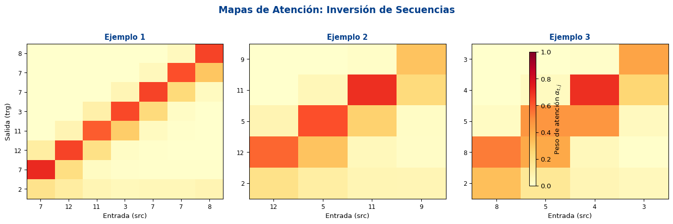
Interpretación
En la tarea de inversión, esperamos ver una diagonal invertida: el primer token generado debe atender al último token de entrada, y viceversa. Los mapas de atención nos permiten interpretar qué aprendió el modelo.
Mapas de Atención en Traducción (Conceptual)
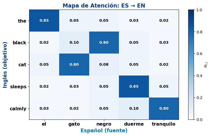
Observaciones interesantes
- “the” atiende a “el” → alineación directa
- “black” atiende a “negro” → el adjetivo se reordenó (español: post-nominal, inglés: pre-nominal)
- Los mapas de atención revelan alineamientos entre idiomas, incluyendo reordenamientos
Efecto en Secuencias Largas
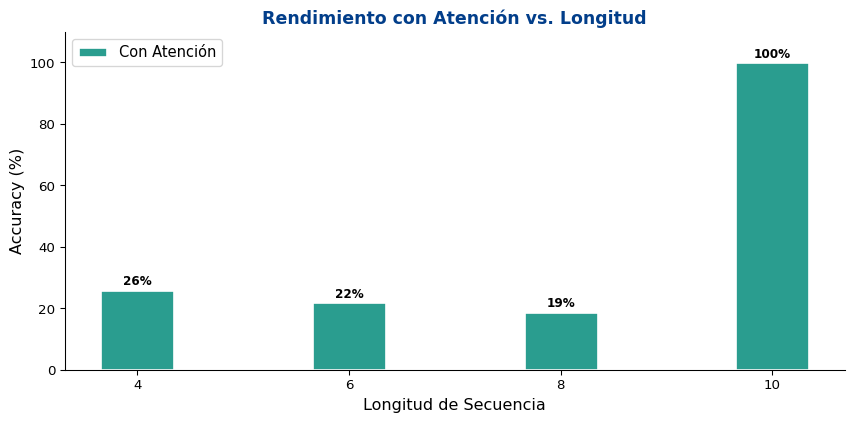
Resultado
La atención mitiga significativamente el problema del cuello de botella. El decoder puede “consultar” directamente los estados relevantes del encoder, sin depender de un solo vector comprimido.
De la Atención al Transformer 🔮
El Camino por Delante
Lo que logramos hoy
- Resolvimos el cuello de botella del vector fijo
- La atención proporciona contexto dinámico en cada paso
- Los mapas de atención son interpretables
- Mejor rendimiento en secuencias largas
Pero todavía hay limitaciones…
- El encoder sigue siendo secuencial (RNN)
- No podemos paralelizar el procesamiento
- ¿Necesitamos la RNN? 🤔
La pregunta revolucionaria (Vaswani et al., 2017)
“Attention Is All You Need”
¿Qué pasaría si elimináramos las RNNs por completo y usáramos solo atención?
→ El Transformer (Semana 9)
Timeline
| Año | Hito |
|---|---|
| 2014 | Seq2Seq (Sutskever, Cho) |
| 2015 | Atención (Bahdanau, Luong) |
| 2017 | Transformer |
| 2018 | BERT, GPT |
| 2020+ | GPT-3, LLMs |
Resumen
Lo Que Aprendimos Hoy
Conceptos
- El cuello de botella del vector fijo limita Seq2Seq
- La atención permite al decoder consultar todos los estados del encoder
- Bahdanau (aditiva): \(v^\top \tanh(Ws + Uh)\)
- Luong (multiplicativa): \(s^\top h\) (producto punto)
- Los pesos \(\alpha_{t,j}\) suman 1 (softmax) y son interpretables
Práctica
BahdanauAttention: MLP con \(W_a\), \(U_a\), \(v_a\)LuongAttention: dot product sin parámetros- Vector de contexto dinámico: \(\mathbf{c}_t = \sum \alpha_{t,j} h_j\)
- Mapas de atención revelan alineamientos
- La atención dot-product evoluciona en el Transformer
Ecuaciones Clave
| Concepto | Ecuación |
|---|---|
| Score (Bahdanau) | \(e_{t,j} = v_a^\top \tanh(W_a s_{t-1} + U_a h_j)\) |
| Score (Luong dot) | \(e_{t,j} = s_t^\top h_j\) |
| Pesos de atención | \(\alpha_{t,j} = \text{softmax}_j(e_{t,j})\) |
| Contexto dinámico | \(\mathbf{c}_t = \sum_{j=1}^{T_x} \alpha_{t,j} \cdot h_j\) |
| Decoder (Bahdanau) | \(s_t = \text{GRU}([\text{emb}(y_{t-1}); \mathbf{c}_t], s_{t-1})\) |
Para la Próxima Semana 📚
Semana 8: Redes Neuronales Convolucionales para NLP
- S1: Convoluciones 1D para texto
- S2: Max Pooling Global vs. Local
- S3: Comparación RNNs vs. CNNs para clasificación
Lectura:
- Kim (2014): Convolutional Neural Networks for Sentence Classification
- Jurafsky & Martin, Cap. 9.3: CNNs for NLP
- Zhang et al. (2015): Character-level Convolutional Networks for Text Classification
Recordatorio:
- Quiz 6 la próxima semana cubre Seq2Seq y Atención 🧮
- Tarea 2: Generador de nombres a nivel de caracteres con LSTM (se publica esta semana)
¿Preguntas? 🙋
¡Gracias!
📧 fsuarez@ucb.edu.bo
🔗 Materiales: github.com/fjsuarez/ucb-nlp
NLP y Análisis Semántico | Semana 7