Redes Neuronales Recurrentes (RNNs)

S2: Gradientes que Desaparecen y la Solución LSTM

Prof. Francisco Suárez

Universidad Católica Boliviana

2026-03-17

Agenda de Hoy

Primera Parte

  1. 🔙 Repaso: RNNs y BPTT
  2. 💀 El problema del gradiente que desaparece (en detalle)
  3. 💡 La intuición detrás de LSTM

Segunda Parte

  1. 🔧 Anatomía de una celda LSTM: las 3 compuertas
  2. 🐍 LSTMs en PyTorch: nn.LSTM
  3. 📊 Comparación práctica: RNN vs. LSTM

Bloque 1: El Problema del Gradiente que Desaparece

Repaso: ¿Cómo Aprende una RNN?

En la sesión anterior vimos la RNN simple (Elman):

\[h_t = \tanh(W_{xh} \cdot x_t + W_{hh} \cdot h_{t-1} + b_h)\]

Para entrenarla usamos Backpropagation Through Time (BPTT): desenrollamos la red y propagamos gradientes hacia atrás por todos los pasos temporales.

Code
graph LR
    x1["x₁"] --> r1["RNN"]
    x2["x₂"] --> r2["RNN"]
    x3["x₃"] --> r3["RNN"]
    x4["x₄"] --> r4["RNN"]
    x5["x₅"] --> r5["RNN"]
    h0["h₀"] --> r1
    r1 -->|"h₁"| r2
    r2 -->|"h₂"| r3
    r3 -->|"h₃"| r4
    r4 -->|"h₄"| r5
    r5 --> L["Loss L"]
    L -.->|"∂L/∂h₅"| r5
    r5 -.->|"∂h₅/∂h₄"| r4
    r4 -.->|"∂h₄/∂h₃"| r3
    r3 -.->|"∂h₃/∂h₂"| r2
    r2 -.->|"∂h₂/∂h₁"| r1
    style r1 fill:#2a9d8f,color:#fff
    style r2 fill:#2a9d8f,color:#fff
    style r3 fill:#2a9d8f,color:#fff
    style r4 fill:#2a9d8f,color:#fff
    style r5 fill:#2a9d8f,color:#fff
    style L fill:#e76f51,color:#fff

El gradiente debe viajar hacia atrás por toda la cadena temporal.

El Producto que Mata los Gradientes

El gradiente del loss respecto a un estado oculto lejano \(h_k\) involucra un producto encadenado:

\[\frac{\partial \mathcal{L}}{\partial h_k} = \frac{\partial \mathcal{L}}{\partial h_T} \prod_{j=k+1}^{T} \frac{\partial h_j}{\partial h_{j-1}}\]

Cada factor del producto es:

\[\frac{\partial h_j}{\partial h_{j-1}} = W_{hh}^T \cdot \text{diag}\left(1 - h_j^2\right)\]

¿Por qué se desvanece?

  • \(\tanh'(x) = 1 - \tanh^2(x)\)
  • Su valor máximo es 1 (en \(x=0\)), y cae rápido
  • Multiplicar muchos valores \(< 1\) → resultado exponencialmente pequeño

Analogía: el juego del teléfono

Imagina pasar un mensaje por 30 personas:

  • Cada persona “atenúa” el mensaje un poco
  • Al final, el mensaje original está irreconocible
  • Los gradientes sufren el mismo destino

Demostración Numérica

import numpy as np
import matplotlib.pyplot as plt

# Simular la multiplicación repetida de la derivada de tanh
# La derivada de tanh está en (0, 1], típicamente ~0.5 para activaciones moderadas

np.random.seed(42)
T = 50  # pasos temporales

# Simulamos el producto de los factores del gradiente
gradient_magnitudes = []
g = 1.0
tanh_derivs = []
for t in range(T):
    # Valor típico de tanh'(h) para activaciones moderadas
    d = np.random.uniform(0.1, 0.7)
    tanh_derivs.append(d)
    g *= d * 0.9  # factor de W_hh incluido
    gradient_magnitudes.append(g)

print(f"Gradiente después de 10 pasos: {gradient_magnitudes[9]:.2e}")
print(f"Gradiente después de 20 pasos: {gradient_magnitudes[19]:.2e}")
print(f"Gradiente después de 30 pasos: {gradient_magnitudes[29]:.2e}")
print(f"Gradiente después de 50 pasos: {gradient_magnitudes[49]:.2e}")
Gradiente después de 10 pasos: 1.42e-05
Gradiente después de 20 pasos: 2.63e-11
Gradiente después de 30 pasos: 7.74e-17
Gradiente después de 50 pasos: 1.98e-27

La Consecuencia Práctica

El gradiente se vuelve tan pequeño que los pesos no se actualizan. La red no puede aprender dependencias a largo plazo — no “recuerda” lo que vio hace 20+ pasos.

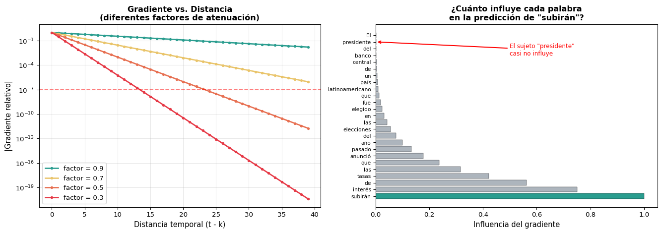
Visualización: Gradiente vs. Distancia Temporal

Code
import numpy as np
import matplotlib.pyplot as plt

fig, axes = plt.subplots(1, 2, figsize=(14, 5))

T = 40
# Izq: diferentes factores de atenuación
factors = [0.9, 0.7, 0.5, 0.3]
colors = ['#2a9d8f', '#e9c46a', '#e76f51', '#e63946']

for factor, color in zip(factors, colors):
    grads = [factor**t for t in range(T)]
    axes[0].plot(range(T), grads, '-o', color=color, label=f'factor = {factor}', markersize=3, linewidth=2)

axes[0].set_xlabel('Distancia temporal (t - k)', fontsize=11)
axes[0].set_ylabel('|Gradiente relativo|', fontsize=11)
axes[0].set_title('Gradiente vs. Distancia\n(diferentes factores de atenuación)', fontweight='bold', fontsize=12)
axes[0].legend(fontsize=10)
axes[0].set_yscale('log')
axes[0].grid(True, alpha=0.3)
axes[0].axhline(y=1e-7, color='red', linestyle='--', alpha=0.5, label='Precisión float32')

# Der: ejemplo con texto real
words = ['El', 'presidente', 'del', 'banco', 'central', 'de', 'un', 'país',
         'latinoamericano', 'que', 'fue', 'elegido', 'en', 'las', 'elecciones',
         'del', 'año', 'pasado', 'anunció', 'que', 'las', 'tasas', 'de', 'interés',
         'subirán']
n = len(words)
memory = np.array([0.75**i for i in range(n)])[::-1]

colors_bar = []
for i, w in enumerate(words):
    if w == 'presidente':
        colors_bar.append('#e76f51')
    elif w == 'subirán':
        colors_bar.append('#2a9d8f')
    else:
        colors_bar.append('#adb5bd')

axes[1].barh(range(n), memory, color=colors_bar, edgecolor='black', linewidth=0.3)
axes[1].set_yticks(range(n))
axes[1].set_yticklabels(words, fontsize=8)
axes[1].set_xlabel('Influencia del gradiente', fontsize=11)
axes[1].set_title('¿Cuánto influye cada palabra\nen la predicción de "subirán"?', fontweight='bold', fontsize=12)
axes[1].invert_yaxis()

axes[1].annotate('El sujeto "presidente"\ncasi no influye', xy=(memory[1], 1), xytext=(0.5, 3),
                arrowprops=dict(arrowstyle='->', color='red', lw=1.5), fontsize=9, color='red')

plt.tight_layout()
plt.show()

Gradient Clipping: Solo Medio Remedio

Gradient clipping (que ya usamos en S1) evita que los gradientes exploten, pero no soluciona el desvanecimiento:

# Solo previene explosión, NO desvanecimiento
torch.nn.utils.clip_grad_norm_(model.parameters(), max_norm=1.0)

✅ Lo que sí resuelve

  • Gradientes que explotan (\(\|W_{hh}\| > 1\))
  • Entrenamiento inestable
  • NaN en los pesos

❌ Lo que NO resuelve

  • Gradientes que desaparecen (\(\|W_{hh}\| < 1\))
  • Pérdida de memoria a largo plazo
  • Incapacidad de aprender dependencias lejanas

Necesitamos una solución arquitectónica

No podemos resolver el vanishing gradient con trucos de entrenamiento. Necesitamos cambiar la arquitectura de la red para que los gradientes puedan fluir sin atenuarse.

Bloque 2: La Intuición de LSTM

¿Y Si la Red Pudiera “Decidir” Qué Recordar?

La RNN simple reescribe \(h_t\) completamente en cada paso:

\[h_t = \tanh(W_{xh} x_t + W_{hh} h_{t-1} + b)\]

Esto es como borrar una pizarra y volver a escribir en cada paso temporal.

Lo que hace la RNN simple

  1. Toma \(h_{t-1}\) y \(x_t\)
  2. Calcula un nuevo \(h_t\) desde cero
  3. La info antigua sobrevive solo si \(W_{hh}\) la preserva “accidentalmente”

Lo que querríamos

  1. Mantener información importante del pasado
  2. Olvidar selectivamente lo irrelevante
  3. Agregar nueva información de forma controlada
  4. Que los gradientes fluyan sin atenuarse

Hochreiter & Schmidhuber (1997): ¿Y si añadimos una “autopista” para la información, con compuertas que regulen el flujo?

Así nace la Long Short-Term Memory (LSTM).

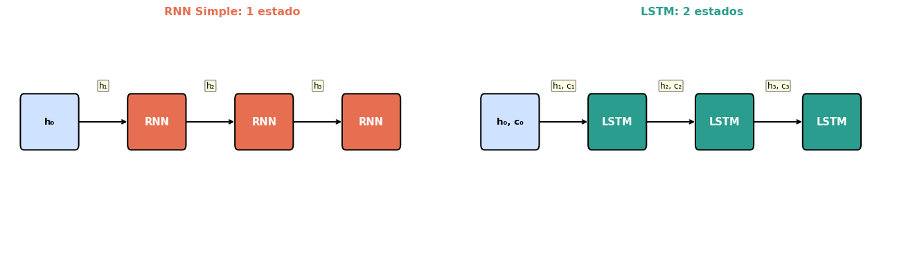
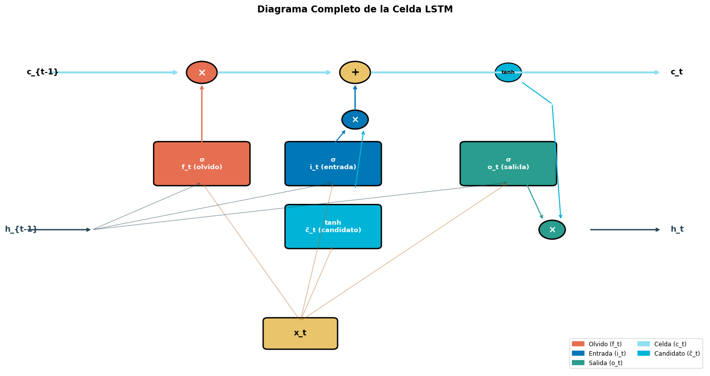
La Idea Clave: La Celda de Memoria

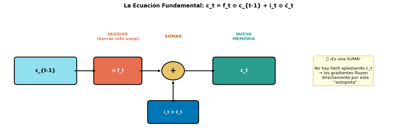
La LSTM introduce un segundo vector de estado: la celda de memoria \(c_t\).

Code
import matplotlib.pyplot as plt
import matplotlib.patches as mpatches

fig, axes = plt.subplots(1, 2, figsize=(14, 4))

def draw_chain(ax, title, labels, edge_labels, color, title_color):
    ax.set_xlim(-0.5, 10)
    ax.set_ylim(-0.5, 3)
    ax.axis('off')
    positions = [(0.5, 1.5), (3, 1.5), (5.5, 1.5), (8, 1.5)]
    # Draw boxes
    for i, (x, y) in enumerate(positions):
        if i == 0:  # initial state
            rect = mpatches.FancyBboxPatch((x-0.6, y-0.35), 1.2, 0.7,
                boxstyle="round,pad=0.08", facecolor='#cfe2ff', edgecolor='black', lw=1.5)
            ax.add_patch(rect)
            ax.text(x, y, labels[i], ha='center', va='center', fontsize=10, fontweight='bold')
        else:
            rect = mpatches.FancyBboxPatch((x-0.6, y-0.35), 1.2, 0.7,
                boxstyle="round,pad=0.08", facecolor=color, edgecolor='black', lw=1.5)
            ax.add_patch(rect)
            ax.text(x, y, labels[i], ha='center', va='center', fontsize=11, color='white', fontweight='bold')
    # Draw arrows with labels
    for i in range(len(positions)-1):
        x1, y1 = positions[i]
        x2, y2 = positions[i+1]
        ax.annotate('', xy=(x2-0.65, y2), xytext=(x1+0.65, y1),
                    arrowprops=dict(arrowstyle='->', color='black', lw=1.5))
        mid_x = (x1 + x2) / 2
        ax.text(mid_x, y1 + 0.55, edge_labels[i], ha='center', va='center', fontsize=9,
                bbox=dict(boxstyle='round,pad=0.15', facecolor='lightyellow', edgecolor='gray', alpha=0.9))
    ax.set_title(title, fontsize=12, fontweight='bold', color=title_color, pad=10)

# RNN Simple
draw_chain(axes[0], 'RNN Simple: 1 estado',
    ['h₀', 'RNN', 'RNN', 'RNN'],
    ['h₁', 'h₂', 'h₃'],
    '#e76f51', '#e76f51')

# LSTM
draw_chain(axes[1], 'LSTM: 2 estados',
    ['h₀, c₀', 'LSTM', 'LSTM', 'LSTM'],
    ['h₁, c₁', 'h₂, c₂', 'h₃, c₃'],
    '#2a9d8f', '#2a9d8f')

plt.tight_layout()
plt.show()

RNN Simple: 1 estado

  • \(h_t\): hace todo (memoria + salida)
  • Transformación no lineal (\(\tanh\)) en cada paso
  • Los gradientes se atenúan

LSTM: 2 estados

  • \(c_t\): memoria a largo plazo (la “autopista”)
  • \(h_t\): memoria de trabajo (salida)
  • La celda \(c_t\) se actualiza aditivamente — ¡sin \(\tanh\) aplastante!

Analogía: La LSTM como un Cuaderno

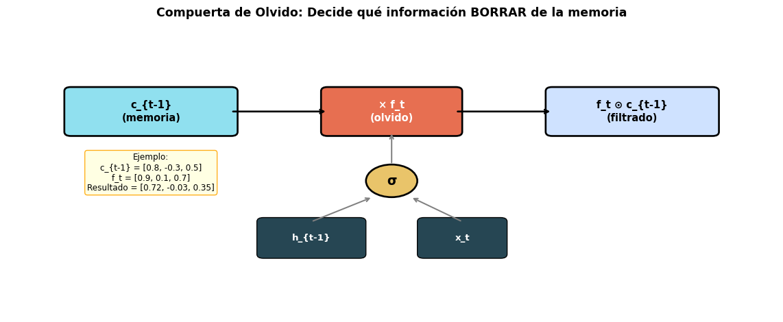
🗑️ Compuerta de Olvido

“¿Qué tachar del cuaderno?”

  • Lee la entrada actual \(x_t\)
  • Decide qué información antigua ya no es relevante
  • Ejemplo: Al ver un nuevo sujeto, olvidar el sujeto anterior

📝 Compuerta de Entrada

“¿Qué escribir en el cuaderno?”

  • Determina qué información nueva es importante
  • La escribe en la celda de memoria
  • Ejemplo: Registrar que el nuevo sujeto es “gato”

📤 Compuerta de Salida

“¿Qué leer del cuaderno ahora?”

  • No toda la memoria es relevante para el paso actual
  • Selecciona qué parte de \(c_t\) usar como salida \(h_t\)
  • Ejemplo: Solo necesito el sujeto para conjugar el verbo

La Clave

Las compuertas son funciones sigmoideas que producen valores entre 0 y 1, actuando como “válvulas” que regulan el flujo de información. Son aprendidas durante el entrenamiento.

Bloque 3: Anatomía de la Celda LSTM

Las Ecuaciones de la LSTM

Una celda LSTM en el paso \(t\) calcula:

Compuertas (sigmoideas)

\[f_t = \sigma(W_f \cdot [h_{t-1}, x_t] + b_f) \quad \text{(olvido)}\] \[i_t = \sigma(W_i \cdot [h_{t-1}, x_t] + b_i) \quad \text{(entrada)}\] \[o_t = \sigma(W_o \cdot [h_{t-1}, x_t] + b_o) \quad \text{(salida)}\]

Celda y estado oculto

\[\tilde{c}_t = \tanh(W_c \cdot [h_{t-1}, x_t] + b_c) \quad \text{(candidato)}\] \[c_t = f_t \odot c_{t-1} + i_t \odot \tilde{c}_t \quad \text{(celda)}\] \[h_t = o_t \odot \tanh(c_t) \quad \text{(salida)}\]

Donde \(\sigma\) es la sigmoide (\(\sigma(x) = \frac{1}{1+e^{-x}}\)) y \(\odot\) es el producto elemento a elemento (Hadamard).

Notación: \([h_{t-1}, x_t]\)

Significa la concatenación de \(h_{t-1} \in \mathbb{R}^{D_h}\) y \(x_t \in \mathbb{R}^d\), resultando en un vector de tamaño \(D_h + d\).

Paso 1: Compuerta de Olvido (\(f_t\))

\[f_t = \sigma(W_f \cdot [h_{t-1}, x_t] + b_f)\]

Code
import matplotlib.pyplot as plt
import matplotlib.patches as mpatches
import numpy as np

fig, ax = plt.subplots(figsize=(12, 5))
ax.set_xlim(-1, 11)
ax.set_ylim(-1, 6)
ax.axis('off')

# c_{t-1} (memoria anterior)
rect = mpatches.FancyBboxPatch((0, 3.5), 2.5, 1, boxstyle="round,pad=0.1",
                                 facecolor='#90e0ef', edgecolor='black', linewidth=2)
ax.add_patch(rect)
ax.text(1.25, 4.0, 'c_{t-1}\n(memoria)', ha='center', va='center', fontsize=11, fontweight='bold')

# Forget gate
rect = mpatches.FancyBboxPatch((4, 3.5), 2, 1, boxstyle="round,pad=0.1",
                                 facecolor='#e76f51', edgecolor='black', linewidth=2)
ax.add_patch(rect)
ax.text(5, 4.0, '× f_t\n(olvido)', ha='center', va='center', fontsize=11, color='white', fontweight='bold')

# Arrow c_{t-1} → forget
ax.annotate('', xy=(4, 4.0), xytext=(2.5, 4.0),
            arrowprops=dict(arrowstyle='->', color='black', lw=2))

# Result
rect = mpatches.FancyBboxPatch((7.5, 3.5), 2.5, 1, boxstyle="round,pad=0.1",
                                 facecolor='#cfe2ff', edgecolor='black', linewidth=2)
ax.add_patch(rect)
ax.text(8.75, 4.0, 'f_t ⊙ c_{t-1}\n(filtrado)', ha='center', va='center', fontsize=11, fontweight='bold')

# Arrow forget → result
ax.annotate('', xy=(7.5, 4.0), xytext=(6, 4.0),
            arrowprops=dict(arrowstyle='->', color='black', lw=2))

# Inputs: h_{t-1}, x_t
rect = mpatches.FancyBboxPatch((3, 0.5), 1.5, 0.8, boxstyle="round,pad=0.1",
                                 facecolor='#264653', edgecolor='black')
ax.add_patch(rect)
ax.text(3.75, 0.9, 'h_{t-1}', ha='center', va='center', fontsize=10, color='white', fontweight='bold')

rect = mpatches.FancyBboxPatch((5.5, 0.5), 1.2, 0.8, boxstyle="round,pad=0.1",
                                 facecolor='#264653', edgecolor='black')
ax.add_patch(rect)
ax.text(6.1, 0.9, 'x_t', ha='center', va='center', fontsize=10, color='white', fontweight='bold')

# Sigma
circle = plt.Circle((5, 2.3), 0.4, facecolor='#e9c46a', edgecolor='black', linewidth=2)
ax.add_patch(circle)
ax.text(5, 2.3, 'σ', ha='center', va='center', fontsize=14, fontweight='bold')

# Arrows inputs → sigma → gate
ax.annotate('', xy=(4.7, 1.9), xytext=(3.75, 1.3),
            arrowprops=dict(arrowstyle='->', color='gray', lw=1.5))
ax.annotate('', xy=(5.3, 1.9), xytext=(6.1, 1.3),
            arrowprops=dict(arrowstyle='->', color='gray', lw=1.5))
ax.annotate('', xy=(5, 3.5), xytext=(5, 2.7),
            arrowprops=dict(arrowstyle='->', color='gray', lw=1.5))

# Example values
ax.text(1.25, 2.5, 'Ejemplo:\nc_{t-1} = [0.8, -0.3, 0.5]\nf_t = [0.9, 0.1, 0.7]\nResultado = [0.72, -0.03, 0.35]',
        ha='center', va='center', fontsize=9,
        bbox=dict(boxstyle='round', facecolor='lightyellow', edgecolor='orange', alpha=0.9))

ax.set_title('Compuerta de Olvido: Decide qué información BORRAR de la memoria',
             fontsize=13, fontweight='bold', pad=15)
plt.tight_layout()
plt.show()
  • \(f_t \approx 1\): mantener esa dimensión de la memoria
  • \(f_t \approx 0\): olvidar esa dimensión

Paso 2: Compuerta de Entrada (\(i_t\)) y Candidato (\(\tilde{c}_t\))

\[i_t = \sigma(W_i \cdot [h_{t-1}, x_t] + b_i) \qquad \tilde{c}_t = \tanh(W_c \cdot [h_{t-1}, x_t] + b_c)\]

Code
import matplotlib.pyplot as plt
import matplotlib.patches as mpatches

fig, ax = plt.subplots(figsize=(12, 5))
ax.set_xlim(-1, 13)
ax.set_ylim(-1, 6)
ax.axis('off')

# Candidate c_tilde
rect = mpatches.FancyBboxPatch((0, 3.5), 2.5, 1, boxstyle="round,pad=0.1",
                                 facecolor='#2a9d8f', edgecolor='black', linewidth=2)
ax.add_patch(rect)
ax.text(1.25, 4.0, 'c̃_t\n(candidato)', ha='center', va='center', fontsize=11, color='white', fontweight='bold')

# Input gate
rect = mpatches.FancyBboxPatch((4, 3.5), 2, 1, boxstyle="round,pad=0.1",
                                 facecolor='#0077b6', edgecolor='black', linewidth=2)
ax.add_patch(rect)
ax.text(5, 4.0, '× i_t\n(entrada)', ha='center', va='center', fontsize=11, color='white', fontweight='bold')

# Arrow candidate → gate
ax.annotate('', xy=(4, 4.0), xytext=(2.5, 4.0),
            arrowprops=dict(arrowstyle='->', color='black', lw=2))

# Result
rect = mpatches.FancyBboxPatch((7.5, 3.5), 2.5, 1, boxstyle="round,pad=0.1",
                                 facecolor='#cfe2ff', edgecolor='black', linewidth=2)
ax.add_patch(rect)
ax.text(8.75, 4.0, 'i_t ⊙ c̃_t\n(info nueva)', ha='center', va='center', fontsize=11, fontweight='bold')

# Arrow gate → result
ax.annotate('', xy=(7.5, 4.0), xytext=(6, 4.0),
            arrowprops=dict(arrowstyle='->', color='black', lw=2))

# Sigma (i_t)
circle = plt.Circle((4.2, 2.3), 0.4, facecolor='#e9c46a', edgecolor='black', linewidth=2)
ax.add_patch(circle)
ax.text(4.2, 2.3, 'σ', ha='center', va='center', fontsize=14, fontweight='bold')

# tanh (c_tilde)
circle2 = plt.Circle((1.25, 2.3), 0.4, facecolor='#90e0ef', edgecolor='black', linewidth=2)
ax.add_patch(circle2)
ax.text(1.25, 2.3, 'tanh', ha='center', va='center', fontsize=10, fontweight='bold')

# Inputs
rect = mpatches.FancyBboxPatch((2, 0.3), 1.5, 0.8, boxstyle="round,pad=0.1",
                                 facecolor='#264653', edgecolor='black')
ax.add_patch(rect)
ax.text(2.75, 0.7, 'h_{t-1}', ha='center', va='center', fontsize=10, color='white', fontweight='bold')

rect = mpatches.FancyBboxPatch((4.5, 0.3), 1.2, 0.8, boxstyle="round,pad=0.1",
                                 facecolor='#264653', edgecolor='black')
ax.add_patch(rect)
ax.text(5.1, 0.7, 'x_t', ha='center', va='center', fontsize=10, color='white', fontweight='bold')

# Arrows
ax.annotate('', xy=(4.0, 1.9), xytext=(2.75, 1.1),
            arrowprops=dict(arrowstyle='->', color='gray', lw=1.2))
ax.annotate('', xy=(4.4, 1.9), xytext=(5.1, 1.1),
            arrowprops=dict(arrowstyle='->', color='gray', lw=1.2))
ax.annotate('', xy=(5, 3.5), xytext=(4.2, 2.7),
            arrowprops=dict(arrowstyle='->', color='gray', lw=1.2))

ax.annotate('', xy=(1.0, 1.9), xytext=(2.75, 1.1),
            arrowprops=dict(arrowstyle='->', color='gray', lw=1.2))
ax.annotate('', xy=(1.5, 1.9), xytext=(5.1, 1.1),
            arrowprops=dict(arrowstyle='->', color='gray', lw=1.2, connectionstyle='arc3,rad=0.3'))
ax.annotate('', xy=(1.25, 3.5), xytext=(1.25, 2.7),
            arrowprops=dict(arrowstyle='->', color='gray', lw=1.2))

# Explanation
ax.text(11, 2.5, 'c̃_t: qué PODRÍA\nescribirse\n(valores -1 a 1)\n\ni_t: cuánto REALMENTE\nescribir\n(valores 0 a 1)',
        ha='center', va='center', fontsize=10,
        bbox=dict(boxstyle='round', facecolor='lightyellow', edgecolor='orange', alpha=0.9))

ax.set_title('Compuerta de Entrada: Decide qué información AGREGAR a la memoria',
             fontsize=13, fontweight='bold', pad=15)
plt.tight_layout()
plt.show()
  • \(\tilde{c}_t\): nueva información candidata (qué podría ser útil)
  • \(i_t\): cuánto de esa información realmente agregar

Paso 3: Actualización de la Celda (\(c_t\))

\[\boxed{c_t = f_t \odot c_{t-1} + i_t \odot \tilde{c}_t}\]

Esta es la ecuación más importante de la LSTM.

Code
import matplotlib.pyplot as plt
import matplotlib.patches as mpatches

fig, ax = plt.subplots(figsize=(14, 4.5))
ax.set_xlim(-0.5, 14)
ax.set_ylim(-0.5, 4.5)
ax.axis('off')

# c_{t-1}
rect = mpatches.FancyBboxPatch((0, 1.5), 2, 1, boxstyle="round,pad=0.1",
                                 facecolor='#90e0ef', edgecolor='black', linewidth=2)
ax.add_patch(rect)
ax.text(1, 2.0, 'c_{t-1}', ha='center', va='center', fontsize=12, fontweight='bold')

# × f_t
rect = mpatches.FancyBboxPatch((2.8, 1.5), 1.5, 1, boxstyle="round,pad=0.1",
                                 facecolor='#e76f51', edgecolor='black', linewidth=2)
ax.add_patch(rect)
ax.text(3.55, 2.0, '⊙ f_t', ha='center', va='center', fontsize=11, color='white', fontweight='bold')

# Arrow
ax.annotate('', xy=(2.8, 2.0), xytext=(2, 2.0),
            arrowprops=dict(arrowstyle='->', color='black', lw=2))

# +
circle = plt.Circle((5.5, 2.0), 0.4, facecolor='#e9c46a', edgecolor='black', linewidth=2)
ax.add_patch(circle)
ax.text(5.5, 2.0, '+', ha='center', va='center', fontsize=18, fontweight='bold')

# Arrow multiply → +
ax.annotate('', xy=(5.1, 2.0), xytext=(4.3, 2.0),
            arrowprops=dict(arrowstyle='->', color='black', lw=2))

# i_t * c_tilde from below
rect = mpatches.FancyBboxPatch((4.7, -0.2), 1.6, 0.8, boxstyle="round,pad=0.1",
                                 facecolor='#0077b6', edgecolor='black', linewidth=2)
ax.add_patch(rect)
ax.text(5.5, 0.2, 'i_t ⊙ c̃_t', ha='center', va='center', fontsize=10, color='white', fontweight='bold')

ax.annotate('', xy=(5.5, 1.6), xytext=(5.5, 0.6),
            arrowprops=dict(arrowstyle='->', color='black', lw=2))

# Arrow + → c_t
ax.annotate('', xy=(7, 2.0), xytext=(5.9, 2.0),
            arrowprops=dict(arrowstyle='->', color='black', lw=2))

# c_t
rect = mpatches.FancyBboxPatch((7, 1.5), 2, 1, boxstyle="round,pad=0.1",
                                 facecolor='#2a9d8f', edgecolor='black', linewidth=2)
ax.add_patch(rect)
ax.text(8, 2.0, 'c_t', ha='center', va='center', fontsize=12, color='white', fontweight='bold')

# Labels
ax.text(3.55, 3.5, 'OLVIDAR\n(borrar info vieja)', ha='center', va='center', fontsize=10, color='#e76f51', fontweight='bold')
ax.text(5.5, 3.5, 'SUMAR', ha='center', va='center', fontsize=10, color='#b5651d', fontweight='bold')
ax.text(8, 3.5, 'NUEVA\nMEMORIA', ha='center', va='center', fontsize=10, color='#2a9d8f', fontweight='bold')

# Explanation box
ax.text(11.5, 2.0,
        '🔑 ¡Es una SUMA!\n\nNo hay tanh aplastando c_t\n→ los gradientes fluyen\n   directamente por esta\n   "autopista"',
        ha='center', va='center', fontsize=10,
        bbox=dict(boxstyle='round', facecolor='lightyellow', edgecolor='orange', alpha=0.9))

ax.set_title('La Ecuación Fundamental: c_t = f_t ⊙ c_{t-1} + i_t ⊙ c̃_t',
             fontsize=13, fontweight='bold', pad=15)
plt.tight_layout()
plt.show()

¿Por Qué Esto Resuelve el Vanishing Gradient?

La celda \(c_t\) se actualiza mediante una suma ponderada, no una transformación no lineal. Si \(f_t \approx 1\), entonces \(c_t \approx c_{t-1}\) — ¡la información pasa sin modificar! Los gradientes fluyen por esta “autopista” sin atenuarse.

Paso 4: Compuerta de Salida (\(o_t\)) y Estado Oculto (\(h_t\))

\[o_t = \sigma(W_o \cdot [h_{t-1}, x_t] + b_o)\] \[h_t = o_t \odot \tanh(c_t)\]

La compuerta de salida determina qué parte de la memoria \(c_t\) se expone como salida:

¿Por qué no usar \(c_t\) directamente?

  • \(c_t\) puede contener información de muchos conceptos acumulados
  • No todo es relevante para la predicción actual
  • \(o_t\) filtra qué aspectos de la memoria son útiles ahora

Ejemplo NLP

Oración: “El gato, que es muy lindo, come

La celda \(c_t\) almacena:

  • Sujeto = “gato” (relevante para conjugar)
  • Adjetivo = “lindo” (no relevante ahora)

\(o_t\) decide: exponer solo la info del sujeto → \(h_t\) sabe conjugar “come” en singular.

Diagrama Completo de la Celda LSTM

Code
import matplotlib.pyplot as plt
import matplotlib.patches as mpatches
import numpy as np

fig, ax = plt.subplots(figsize=(15, 8))
ax.set_xlim(-1, 15)
ax.set_ylim(-2, 9)
ax.axis('off')

# Colors
c_forget = '#e76f51'
c_input = '#0077b6'
c_output = '#2a9d8f'
c_cell = '#90e0ef'
c_hidden = '#264653'
c_sigma = '#e9c46a'

# ====== CELL STATE LINE (top highway) ======
# c_{t-1} →
ax.annotate('', xy=(3, 7.5), xytext=(0, 7.5),
            arrowprops=dict(arrowstyle='->', color=c_cell, lw=3))
ax.text(-0.5, 7.5, 'c_{t-1}', fontsize=12, fontweight='bold', va='center')

# × (forget)
circle = plt.Circle((3.5, 7.5), 0.35, facecolor=c_forget, edgecolor='black', linewidth=2)
ax.add_patch(circle)
ax.text(3.5, 7.5, '×', ha='center', va='center', fontsize=16, color='white', fontweight='bold')

# → + (add)
ax.annotate('', xy=(6.5, 7.5), xytext=(3.85, 7.5),
            arrowprops=dict(arrowstyle='->', color=c_cell, lw=3))
circle = plt.Circle((7, 7.5), 0.35, facecolor=c_sigma, edgecolor='black', linewidth=2)
ax.add_patch(circle)
ax.text(7, 7.5, '+', ha='center', va='center', fontsize=16, fontweight='bold')

# → c_t
ax.annotate('', xy=(14, 7.5), xytext=(7.35, 7.5),
            arrowprops=dict(arrowstyle='->', color=c_cell, lw=3))
ax.text(14.2, 7.5, 'c_t', fontsize=12, fontweight='bold', va='center')

# ====== HIDDEN STATE LINE (bottom) ======
ax.annotate('', xy=(1, 2.5), xytext=(-0.5, 2.5),
            arrowprops=dict(arrowstyle='->', color=c_hidden, lw=2))
ax.text(-1, 2.5, 'h_{t-1}', fontsize=12, fontweight='bold', va='center', color=c_hidden)

# → h_t
ax.annotate('', xy=(14, 2.5), xytext=(12.35, 2.5),
            arrowprops=dict(arrowstyle='->', color=c_hidden, lw=2))
ax.text(14.2, 2.5, 'h_t', fontsize=12, fontweight='bold', va='center', color=c_hidden)

# ====== GATES ======

# -- Forget gate (f_t) --
rect = mpatches.FancyBboxPatch((2.5, 4.0), 2, 1.2, boxstyle="round,pad=0.1",
                                 facecolor=c_forget, edgecolor='black', linewidth=2)
ax.add_patch(rect)
ax.text(3.5, 4.6, \nf_t (olvido)', ha='center', va='center', fontsize=10, color='white', fontweight='bold')
ax.annotate('', xy=(3.5, 7.15), xytext=(3.5, 5.2),
            arrowprops=dict(arrowstyle='->', color=c_forget, lw=2))

# -- Input gate (i_t) --
rect = mpatches.FancyBboxPatch((5.5, 4.0), 2, 1.2, boxstyle="round,pad=0.1",
                                 facecolor=c_input, edgecolor='black', linewidth=2)
ax.add_patch(rect)
ax.text(6.5, 4.6, \ni_t (entrada)', ha='center', va='center', fontsize=10, color='white', fontweight='bold')

# -- Candidate (c_tilde) --
rect = mpatches.FancyBboxPatch((5.5, 2.0), 2, 1.2, boxstyle="round,pad=0.1",
                                 facecolor='#00b4d8', edgecolor='black', linewidth=2)
ax.add_patch(rect)
ax.text(6.5, 2.6, 'tanh\nc̃_t (candidato)', ha='center', va='center', fontsize=10, color='white', fontweight='bold')

# i_t × c_tilde → multiplication
circle = plt.Circle((7, 6.0), 0.3, facecolor=c_input, edgecolor='black', linewidth=2)
ax.add_patch(circle)
ax.text(7, 6.0, '×', ha='center', va='center', fontsize=14, color='white', fontweight='bold')

ax.annotate('', xy=(6.8, 5.7), xytext=(6.5, 5.2),
            arrowprops=dict(arrowstyle='->', color=c_input, lw=1.5))
ax.annotate('', xy=(7, 3.2), xytext=(6.5, 3.2),
            arrowprops=dict(arrowstyle='-', color='#00b4d8', lw=1.5))
ax.annotate('', xy=(7.2, 5.7), xytext=(7, 3.8),
            arrowprops=dict(arrowstyle='->', color='#00b4d8', lw=1.5))
ax.annotate('', xy=(7, 7.15), xytext=(7, 6.3),
            arrowprops=dict(arrowstyle='->', color=c_input, lw=2))

# -- Output gate (o_t) --
rect = mpatches.FancyBboxPatch((9.5, 4.0), 2, 1.2, boxstyle="round,pad=0.1",
                                 facecolor=c_output, edgecolor='black', linewidth=2)
ax.add_patch(rect)
ax.text(10.5, 4.6, \no_t (salida)', ha='center', va='center', fontsize=10, color='white', fontweight='bold')

# tanh on cell → output gate
circle = plt.Circle((10.5, 7.5), 0.3, facecolor='#00b4d8', edgecolor='black', linewidth=1.5)
ax.add_patch(circle)
ax.text(10.5, 7.5, 'tanh', ha='center', va='center', fontsize=8, fontweight='bold')

# tanh → × with o_t
circle2 = plt.Circle((11.5, 2.5), 0.3, facecolor=c_output, edgecolor='black', linewidth=2)
ax.add_patch(circle2)
ax.text(11.5, 2.5, '×', ha='center', va='center', fontsize=14, color='white', fontweight='bold')

ax.annotate('', xy=(11.5, 6.5), xytext=(10.8, 7.2),
            arrowprops=dict(arrowstyle='-', color='#00b4d8', lw=1.5))
ax.annotate('', xy=(11.7, 2.8), xytext=(11.5, 6.5),
            arrowprops=dict(arrowstyle='->', color='#00b4d8', lw=1.5))
ax.annotate('', xy=(11.3, 2.8), xytext=(10.5, 5.2),
            arrowprops=dict(arrowstyle='->', color=c_output, lw=1.5))

# h_{t-1} → gates (fan out from bottom)
for gx in [3.5, 6.5, 10.5]:
    ax.annotate('', xy=(gx, 4.0), xytext=(1, 2.5),
                arrowprops=dict(arrowstyle='->', color=c_hidden, lw=1, alpha=0.5))

# x_t
rect = mpatches.FancyBboxPatch((5, -1.2), 1.5, 0.8, boxstyle="round,pad=0.1",
                                 facecolor='#e9c46a', edgecolor='black', linewidth=2)
ax.add_patch(rect)
ax.text(5.75, -0.8, 'x_t', ha='center', va='center', fontsize=12, fontweight='bold')

for gx in [3.5, 6.5, 10.5]:
    ax.annotate('', xy=(gx, 4.0), xytext=(5.75, -0.4),
                arrowprops=dict(arrowstyle='->', color='#b5651d', lw=1, alpha=0.5))

# Also x_t → candidate
ax.annotate('', xy=(6.5, 2.0), xytext=(5.75, -0.4),
            arrowprops=dict(arrowstyle='->', color='#b5651d', lw=1, alpha=0.5))

# Title and legend
ax.set_title('Diagrama Completo de la Celda LSTM', fontsize=14, fontweight='bold', pad=20)

# Legend
legend_items = [
    mpatches.Patch(color=c_forget, label='Olvido (f_t)'),
    mpatches.Patch(color=c_input, label='Entrada (i_t)'),
    mpatches.Patch(color=c_output, label='Salida (o_t)'),
    mpatches.Patch(color=c_cell, label='Celda (c_t)'),
    mpatches.Patch(color='#00b4d8', label='Candidato (c̃_t)'),
]
ax.legend(handles=legend_items, loc='lower right', fontsize=9, ncol=2)

plt.tight_layout()
plt.show()

¿Por Qué la LSTM Resuelve el Vanishing Gradient?

La clave está en cómo fluyen los gradientes por la celda \(c_t\):

\[c_t = f_t \odot c_{t-1} + i_t \odot \tilde{c}_t\]

\[\frac{\partial c_t}{\partial c_{t-1}} = f_t\]

RNN Simple

\[\frac{\partial h_t}{\partial h_{t-1}} = W_{hh}^T \cdot \text{diag}(1-h_t^2)\]

  • Multiplicación por \(W_{hh}\) y \(\tanh'\) en cada paso
  • Los gradientes se atenúan exponencialmente
  • Imposible aprender dependencias largas

LSTM

\[\frac{\partial c_t}{\partial c_{t-1}} = f_t \quad (\text{sin } W_{hh}, \text{ sin } \tanh')\]

  • Solo multiplicación por \(f_t \in (0, 1)\)
  • Si \(f_t \approx 1\): gradiente pasa intacto
  • La red aprende a mantener \(f_t\) alto para dependencias largas

La “Autopista” del Gradiente

La celda \(c_t\) actúa como un Constant Error Carousel (CEC) — una autopista por donde la información y los gradientes pueden fluir sin degradarse, siempre que \(f_t\) se mantenga cercano a 1.

¿Cuántos Parámetros Tiene una LSTM?

Una LSTM tiene 4 veces más parámetros que una RNN simple (4 conjuntos de pesos: \(f\), \(i\), \(o\), \(\tilde{c}\)):

import torch.nn as nn

input_size = 100   # embedding dim
hidden_size = 128  # estado oculto

rnn = nn.RNN(input_size, hidden_size, batch_first=True)
lstm = nn.LSTM(input_size, hidden_size, batch_first=True)

rnn_params = sum(p.numel() for p in rnn.parameters())
lstm_params = sum(p.numel() for p in lstm.parameters())

print(f"RNN  parámetros: {rnn_params:>8,}")
print(f"LSTM parámetros: {lstm_params:>8,}")
print(f"Ratio LSTM/RNN:  {lstm_params/rnn_params:.1f}x")
RNN  parámetros:   29,440
LSTM parámetros:  117,760
Ratio LSTM/RNN:  4.0x
Componente RNN Simple LSTM
Pesos entrada→oculto \(W_{xh}: D_h \times d\) \(W_{xi}, W_{xf}, W_{xo}, W_{xc}: 4 \times D_h \times d\)
Pesos oculto→oculto \(W_{hh}: D_h \times D_h\) \(W_{hi}, W_{hf}, W_{ho}, W_{hc}: 4 \times D_h \times D_h\)
Biases \(b_h: D_h\) \(b_i, b_f, b_o, b_c: 4 \times D_h\)
Total \(D_h(d + D_h + 1)\) \(4 \times D_h(d + D_h + 1)\)

Bloque 4: LSTM en PyTorch

nn.LSTM Paso a Paso

import torch
import torch.nn as nn

# Definir LSTM
lstm = nn.LSTM(
    input_size=64,      # dimensión de entrada (embedding_dim)
    hidden_size=128,    # dimensión del estado oculto
    num_layers=1,       # capas apiladas
    batch_first=True    # entrada: (batch, seq_len, input_size)
)

# Entrada: batch de 3 secuencias de longitud 10
x = torch.randn(3, 10, 64)  # (batch=3, seq_len=10, input_size=64)

# Forward pass — LSTM devuelve output, (h_n, c_n)
output, (h_n, c_n) = lstm(x)

print(f"Entrada:      {x.shape}         →  (batch, seq_len, input)")
print(f"Salida:       {output.shape}   →  (batch, seq_len, hidden)")
print(f"h_n (oculto): {h_n.shape}       →  (layers, batch, hidden)")
print(f"c_n (celda):  {c_n.shape}       →  (layers, batch, hidden)")
print(f"\n¿output[:,-1,:] == h_n[0]?  {torch.allclose(output[:, -1, :], h_n[0])}")
Entrada:      torch.Size([3, 10, 64])         →  (batch, seq_len, input)
Salida:       torch.Size([3, 10, 128])   →  (batch, seq_len, hidden)
h_n (oculto): torch.Size([1, 3, 128])       →  (layers, batch, hidden)
c_n (celda):  torch.Size([1, 3, 128])       →  (layers, batch, hidden)

¿output[:,-1,:] == h_n[0]?  True

Diferencia clave con nn.RNN

  • nn.RNN.forward()output, h_n
  • nn.LSTM.forward()output, (h_n, c_n) — devuelve dos estados

Clasificador de Texto: RNN vs. LSTM

import torch
import torch.nn as nn

class LSTMClassifier(nn.Module):
    """Clasificador Many-to-One con LSTM."""
    def __init__(self, vocab_size, embed_dim, hidden_dim, n_classes, padding_idx=0):
        super().__init__()
        self.embedding = nn.Embedding(vocab_size, embed_dim, padding_idx=padding_idx)
        self.lstm = nn.LSTM(embed_dim, hidden_dim, batch_first=True)
        self.fc = nn.Linear(hidden_dim, n_classes)
        self.dropout = nn.Dropout(0.3)

    def forward(self, x):
        emb = self.embedding(x)                  # (batch, seq_len, embed_dim)
        output, (h_n, c_n) = self.lstm(emb)      # h_n: (1, batch, hidden)
        h_last = h_n.squeeze(0)                   # (batch, hidden)
        h_last = self.dropout(h_last)
        logits = self.fc(h_last)                  # (batch, n_classes)
        return logits

model_lstm = LSTMClassifier(vocab_size=10000, embed_dim=100, hidden_dim=128, n_classes=2)
print(model_lstm)
print(f"\nParámetros: {sum(p.numel() for p in model_lstm.parameters()):,}")
LSTMClassifier(
  (embedding): Embedding(10000, 100, padding_idx=0)
  (lstm): LSTM(100, 128, batch_first=True)
  (fc): Linear(in_features=128, out_features=2, bias=True)
  (dropout): Dropout(p=0.3, inplace=False)
)

Parámetros: 1,118,018

Diferencia mínima en el código — solo cambiamos nn.RNN por nn.LSTM y desempaquetamos (h_n, c_n).

LSTM Multicapa (Stacked LSTM)

# LSTM con 2 capas + dropout entre capas
lstm_stacked = nn.LSTM(
    input_size=64,
    hidden_size=128,
    num_layers=2,
    batch_first=True,
    dropout=0.3      # dropout entre capas (no en la última)
)

x = torch.randn(3, 10, 64)
output, (h_n, c_n) = lstm_stacked(x)

print(f"Salida:  {output.shape}   →  salida de la ÚLTIMA capa")
print(f"h_n:     {h_n.shape}   →  h final de CADA capa")
print(f"c_n:     {c_n.shape}   →  c final de CADA capa")
print(f"\nPara clasificación, usamos h_n[-1]: {h_n[-1].shape}")
Salida:  torch.Size([3, 10, 128])   →  salida de la ÚLTIMA capa
h_n:     torch.Size([2, 3, 128])   →  h final de CADA capa
c_n:     torch.Size([2, 3, 128])   →  c final de CADA capa

Para clasificación, usamos h_n[-1]: torch.Size([3, 128])
Code
graph LR
    subgraph "Capa 1"
        x1["x₁"] --> l11["LSTM L1"]
        x2["x₂"] --> l12["LSTM L1"]
        x3["x₃"] --> l13["LSTM L1"]
        l11 -->|"h¹₁,c¹₁"| l12
        l12 -->|"h¹₂,c¹₂"| l13
    end
    subgraph "Capa 2"
        l11 -->|"h¹₁"| l21["LSTM L2"]
        l12 -->|"h¹₂"| l22["LSTM L2"]
        l13 -->|"h¹₃"| l23["LSTM L2"]
        l21 -->|"h²₁,c²₁"| l22
        l22 -->|"h²₂,c²₂"| l23
    end
    style l11 fill:#2a9d8f,color:#fff
    style l12 fill:#2a9d8f,color:#fff
    style l13 fill:#2a9d8f,color:#fff
    style l21 fill:#264653,color:#fff
    style l22 fill:#264653,color:#fff
    style l23 fill:#264653,color:#fff

Bloque 5: Comparación Práctica RNN vs. LSTM

Experimento: Clasificación de Texto

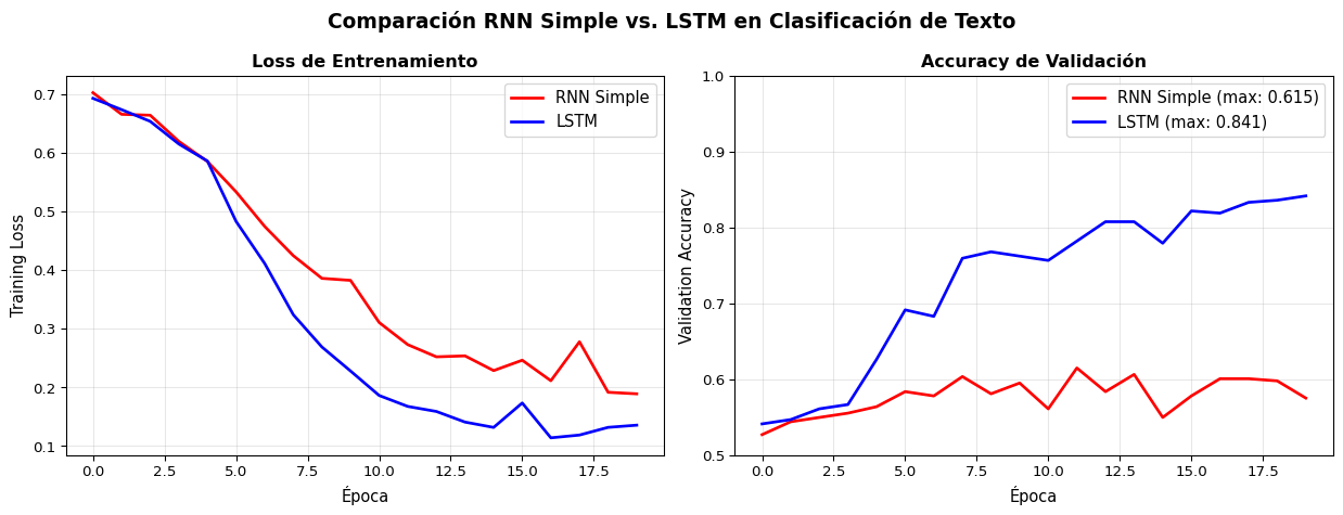
Entrenemos ambos modelos en el mismo dataset y comparemos:

Code
import torch
import torch.nn as nn
import numpy as np
from sklearn.datasets import fetch_20newsgroups
from sklearn.model_selection import train_test_split
from collections import Counter
import matplotlib.pyplot as plt

# ---------- Datos ----------
categories = ['sci.space', 'talk.politics.misc']
data = fetch_20newsgroups(subset='all', categories=categories, remove=('headers', 'footers'))
texts, labels = data.data, data.target

def simple_tokenize(text, max_len=100):
    return text.lower().split()[:max_len]

all_tokens = [t for text in texts for t in simple_tokenize(text)]
word_counts = Counter(all_tokens)
vocab_list = ['<pad>', '<unk>'] + [w for w, c in word_counts.most_common(5000)]
word2idx = {w: i for i, w in enumerate(vocab_list)}

def encode(text, max_len=100):
    tokens = simple_tokenize(text, max_len)
    ids = [word2idx.get(t, 1) for t in tokens]
    ids += [0] * (max_len - len(ids))
    return ids

X = torch.tensor([encode(t) for t in texts])
y = torch.tensor(labels)
X_train, X_val, y_train, y_val = train_test_split(X, y, test_size=0.2, random_state=42)
train_ds = torch.utils.data.TensorDataset(X_train, y_train)
train_loader = torch.utils.data.DataLoader(train_ds, batch_size=32, shuffle=True)

# ---------- Modelos ----------
class SimpleRNN(nn.Module):
    def __init__(self, vocab_size, embed_dim, hidden_dim, n_classes):
        super().__init__()
        self.embedding = nn.Embedding(vocab_size, embed_dim, padding_idx=0)
        self.rnn = nn.RNN(embed_dim, hidden_dim, batch_first=True)
        self.fc = nn.Linear(hidden_dim, n_classes)
        self.dropout = nn.Dropout(0.3)

    def forward(self, x):
        emb = self.embedding(x)
        _, h_n = self.rnn(emb)
        h = self.dropout(h_n.squeeze(0))
        return self.fc(h)

class LSTM_Model(nn.Module):
    def __init__(self, vocab_size, embed_dim, hidden_dim, n_classes):
        super().__init__()
        self.embedding = nn.Embedding(vocab_size, embed_dim, padding_idx=0)
        self.lstm = nn.LSTM(embed_dim, hidden_dim, batch_first=True)
        self.fc = nn.Linear(hidden_dim, n_classes)
        self.dropout = nn.Dropout(0.3)

    def forward(self, x):
        emb = self.embedding(x)
        _, (h_n, _) = self.lstm(emb)
        h = self.dropout(h_n.squeeze(0))
        return self.fc(h)

# ---------- Entrenamiento ----------
def train_model(model, name, epochs=20):
    optimizer = torch.optim.Adam(model.parameters(), lr=0.001)
    criterion = nn.CrossEntropyLoss()
    train_losses, val_accs = [], []

    for epoch in range(epochs):
        model.train()
        epoch_loss = 0
        for xb, yb in train_loader:
            optimizer.zero_grad()
            loss = criterion(model(xb), yb)
            loss.backward()
            torch.nn.utils.clip_grad_norm_(model.parameters(), 1.0)
            optimizer.step()
            epoch_loss += loss.item()
        train_losses.append(epoch_loss / len(train_loader))

        model.eval()
        with torch.no_grad():
            val_acc = (model(X_val).argmax(1) == y_val).float().mean().item()
            val_accs.append(val_acc)

    return train_losses, val_accs

torch.manual_seed(42)
rnn_model = SimpleRNN(len(vocab_list), 64, 64, 2)
rnn_losses, rnn_accs = train_model(rnn_model, "RNN")

torch.manual_seed(42)
lstm_model = LSTM_Model(len(vocab_list), 64, 64, 2)
lstm_losses, lstm_accs = train_model(lstm_model, "LSTM")

# ---------- Gráficas ----------
fig, axes = plt.subplots(1, 2, figsize=(13, 5))

axes[0].plot(rnn_losses, 'r-', linewidth=2, label='RNN Simple')
axes[0].plot(lstm_losses, 'b-', linewidth=2, label='LSTM')
axes[0].set_xlabel('Época', fontsize=11)
axes[0].set_ylabel('Training Loss', fontsize=11)
axes[0].set_title('Loss de Entrenamiento', fontweight='bold', fontsize=12)
axes[0].legend(fontsize=11)
axes[0].grid(True, alpha=0.3)

axes[1].plot(rnn_accs, 'r-', linewidth=2, label=f'RNN Simple (max: {max(rnn_accs):.3f})')
axes[1].plot(lstm_accs, 'b-', linewidth=2, label=f'LSTM (max: {max(lstm_accs):.3f})')
axes[1].set_xlabel('Época', fontsize=11)
axes[1].set_ylabel('Validation Accuracy', fontsize=11)
axes[1].set_title('Accuracy de Validación', fontweight='bold', fontsize=12)
axes[1].legend(fontsize=11)
axes[1].set_ylim(0.5, 1.0)
axes[1].grid(True, alpha=0.3)

plt.suptitle('Comparación RNN Simple vs. LSTM en Clasificación de Texto',
             fontsize=14, fontweight='bold')
plt.tight_layout()
plt.show()

rnn_p = sum(p.numel() for p in rnn_model.parameters())
lstm_p = sum(p.numel() for p in lstm_model.parameters())
print(f"\nRNN  — Params: {rnn_p:>8,} | Best Val Acc: {max(rnn_accs):.4f}")
print(f"LSTM — Params: {lstm_p:>8,} | Best Val Acc: {max(lstm_accs):.4f}")

RNN  — Params:  328,578 | Best Val Acc: 0.6147
LSTM — Params:  353,538 | Best Val Acc: 0.8414

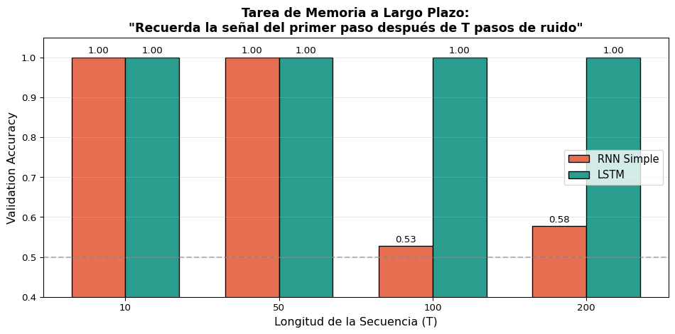
Experimento: Memoria a Largo Plazo

La entrada tiene 2 canales: señal (\(\pm 1\) en canal 0, solo en \(t=0\)) y ruido (gaussiano en canal 1, en todo momento). ¿Puede la red recordar la señal después de \(T\) pasos?

Code
import torch
import torch.nn as nn
import numpy as np
import matplotlib.pyplot as plt

# Entrada bidimensional:
#   Canal 0: señal +1/-1 SOLO en t=0, ceros después
#   Canal 1: ruido gaussiano (std=1) en TODOS los pasos
# El ruido constante empuja el estado oculto de la RNN en cada paso,
# borrando progresivamente la señal. La LSTM puede cerrar la compuerta
# de entrada (i_t ≈ 0) y preservar la señal en la celda c_t.

hidden_dim = 48
n_train, n_val = 4000, 500
seq_lengths = [10, 50, 100, 200]

results = {'RNN': [], 'LSTM': []}

class MemoryModel(nn.Module):
    def __init__(self, model_type):
        super().__init__()
        if model_type == 'RNN':
            self.rnn = nn.RNN(2, hidden_dim, batch_first=True)
        else:
            self.rnn = nn.LSTM(2, hidden_dim, batch_first=True)
            # Truco de Jozefowicz et al. (2015): inicializar el bias
            # de la compuerta de olvido en 1.0 para que f_t empiece ≈ 0.73
            for name, p in self.rnn.named_parameters():
                if 'bias' in name:
                    n = p.size(0)
                    p.data[n//4:n//2].fill_(1.0)
        self.fc = nn.Linear(hidden_dim, 2)
        self.model_type = model_type

    def forward(self, x):
        out = self.rnn(x)
        if self.model_type == 'LSTM':
            _, (h_n, _) = out
        else:
            _, h_n = out
        return self.fc(h_n.squeeze(0))

for T in seq_lengths:
    labels = torch.randint(0, 2, (n_train + n_val,))
    X = torch.zeros(n_train + n_val, T, 2)
    X[:, 0, 0] = labels.float() * 2 - 1       # señal en canal 0, t=0
    X[:, :, 1] = torch.randn(n_train + n_val, T)  # ruido en canal 1
    y = labels.long()

    X_train, X_val = X[:n_train], X[n_train:]
    y_train, y_val = y[:n_train], y[n_train:]
    loader = torch.utils.data.DataLoader(
        torch.utils.data.TensorDataset(X_train, y_train), batch_size=128, shuffle=True)

    for model_type in ['RNN', 'LSTM']:
        torch.manual_seed(42)
        model = MemoryModel(model_type)
        optimizer = torch.optim.Adam(model.parameters(), lr=0.001)
        criterion = nn.CrossEntropyLoss()

        best_acc = 0.0
        for epoch in range(80):
            model.train()
            for xb, yb in loader:
                optimizer.zero_grad()
                loss = criterion(model(xb), yb)
                loss.backward()
                torch.nn.utils.clip_grad_norm_(model.parameters(), 1.0)
                optimizer.step()
            model.eval()
            with torch.no_grad():
                acc = (model(X_val).argmax(1) == y_val).float().mean().item()
                best_acc = max(best_acc, acc)

        results[model_type].append(best_acc)

# Gráfica
fig, ax = plt.subplots(figsize=(10, 5))
x_pos = np.arange(len(seq_lengths))
width = 0.35

bars1 = ax.bar(x_pos - width/2, results['RNN'], width, label='RNN Simple',
               color='#e76f51', edgecolor='black')
bars2 = ax.bar(x_pos + width/2, results['LSTM'], width, label='LSTM',
               color='#2a9d8f', edgecolor='black')

ax.set_xlabel('Longitud de la Secuencia (T)', fontsize=12)
ax.set_ylabel('Validation Accuracy', fontsize=12)
ax.set_title('Tarea de Memoria a Largo Plazo:\n"Recuerda la señal del primer paso después de T pasos de ruido"',
             fontsize=13, fontweight='bold')
ax.set_xticks(x_pos)
ax.set_xticklabels([str(t) for t in seq_lengths])
ax.legend(fontsize=11)
ax.set_ylim(0.4, 1.05)
ax.axhline(y=0.5, color='gray', linestyle='--', alpha=0.5)
ax.grid(True, alpha=0.3, axis='y')

for bar in bars1:
    ax.text(bar.get_x() + bar.get_width()/2., bar.get_height() + 0.01,
            f'{bar.get_height():.2f}', ha='center', fontsize=10)
for bar in bars2:
    ax.text(bar.get_x() + bar.get_width()/2., bar.get_height() + 0.01,
            f'{bar.get_height():.2f}', ha='center', fontsize=10)

plt.tight_layout()
plt.show()

Resultado Clave

El canal de ruido constante empuja el estado oculto de la RNN en cada paso, borrando la señal. La LSTM aprende a cerrar la compuerta de entrada (\(i_t \approx 0\)) para el ruido y mantener la compuerta de olvido (\(f_t \approx 1\)), preservando la señal en \(c_t\).

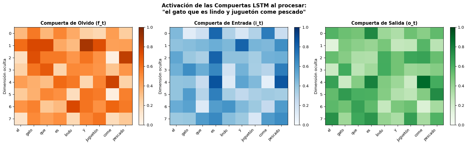
Visualización: Las Compuertas en Acción

Code
import torch
import torch.nn as nn
import matplotlib.pyplot as plt
import numpy as np

# Crear un LSTM y procesar una oración paso a paso
torch.manual_seed(42)

vocab = {'<pad>': 0, 'el': 1, 'gato': 2, 'que': 3, 'es': 4, 'lindo': 5,
         'y': 6, 'juguetón': 7, 'come': 8, 'pescado': 9}
embed_dim = 16
hidden_dim = 8

embedding = nn.Embedding(len(vocab), embed_dim)
lstm_cell = nn.LSTMCell(embed_dim, hidden_dim)

sentence = ['el', 'gato', 'que', 'es', 'lindo', 'y', 'juguetón', 'come', 'pescado']
indices = torch.tensor([vocab[w] for w in sentence])
embs = embedding(indices)

# Registrar las compuertas
h = torch.zeros(1, hidden_dim)
c = torch.zeros(1, hidden_dim)

all_f, all_i, all_o = [], [], []

for t in range(len(sentence)):
    x = embs[t].unsqueeze(0)
    # Manualmente calcular las compuertas para visualizar
    gates = torch.mm(x, lstm_cell.weight_ih.T) + torch.mm(h, lstm_cell.weight_hh.T) + lstm_cell.bias_ih + lstm_cell.bias_hh
    i_gate = torch.sigmoid(gates[:, :hidden_dim])
    f_gate = torch.sigmoid(gates[:, hidden_dim:2*hidden_dim])
    c_cand = torch.tanh(gates[:, 2*hidden_dim:3*hidden_dim])
    o_gate = torch.sigmoid(gates[:, 3*hidden_dim:])

    c = f_gate * c + i_gate * c_cand
    h = o_gate * torch.tanh(c)

    all_f.append(f_gate.detach().numpy().flatten())
    all_i.append(i_gate.detach().numpy().flatten())
    all_o.append(o_gate.detach().numpy().flatten())

all_f = np.array(all_f)
all_i = np.array(all_i)
all_o = np.array(all_o)

fig, axes = plt.subplots(1, 3, figsize=(16, 5))

for ax, data, title, cmap in [
    (axes[0], all_f, 'Compuerta de Olvido (f_t)', 'Oranges'),
    (axes[1], all_i, 'Compuerta de Entrada (i_t)', 'Blues'),
    (axes[2], all_o, 'Compuerta de Salida (o_t)', 'Greens'),
]:
    im = ax.imshow(data.T, aspect='auto', cmap=cmap, vmin=0, vmax=1)
    ax.set_xticks(range(len(sentence)))
    ax.set_xticklabels(sentence, rotation=45, ha='right', fontsize=9)
    ax.set_ylabel('Dimensión oculta', fontsize=10)
    ax.set_title(title, fontweight='bold', fontsize=11)
    plt.colorbar(im, ax=ax, fraction=0.046)

plt.suptitle('Activación de las Compuertas LSTM al procesar:\n"el gato que es lindo y juguetón come pescado"',
             fontsize=13, fontweight='bold')
plt.tight_layout()
plt.show()

Interpretando las Compuertas

Los valores cercanos a 1 (colores oscuros) indican que la compuerta está “abierta”. Observa cómo diferentes dimensiones del estado oculto se activan para diferentes palabras — la red aprende a especializar cada dimensión.

Bloque 6: Resumen y Comparación

Tabla Comparativa: RNN vs. LSTM

Característica RNN Simple LSTM
Estados \(h_t\) (1 estado) \(h_t, c_t\) (2 estados)
Actualización \(h_t = \tanh(W_{xh}x_t + W_{hh}h_{t-1})\) \(c_t = f_t \odot c_{t-1} + i_t \odot \tilde{c}_t\)
Compuertas Ninguna 3 (\(f_t, i_t, o_t\))
Parámetros \(D_h(d + D_h + 1)\) \(4 \times D_h(d + D_h + 1)\)
Memoria ~10-20 tokens ~100-200+ tokens
Gradientes Se desvanecen rápido Fluyen por la “autopista” \(c_t\)
Velocidad Más rápido ~4× más lento
Cuándo usar Secuencias cortas, tareas simples Dependencias largas, producción

Resumen de Ecuaciones LSTM

\[\boxed{f_t = \sigma(W_f [h_{t-1}, x_t] + b_f)} \quad \text{¿Qué olvidar?}\]

\[\boxed{i_t = \sigma(W_i [h_{t-1}, x_t] + b_i)} \quad \text{¿Qué escribir?}\]

\[\boxed{\tilde{c}_t = \tanh(W_c [h_{t-1}, x_t] + b_c)} \quad \text{Info candidata}\]

\[\boxed{c_t = f_t \odot c_{t-1} + i_t \odot \tilde{c}_t} \quad \text{Nueva memoria}\]

\[\boxed{o_t = \sigma(W_o [h_{t-1}, x_t] + b_o)} \quad \text{¿Qué leer?}\]

\[\boxed{h_t = o_t \odot \tanh(c_t)} \quad \text{Salida}\]

Resumen

Lo Que Aprendimos Hoy

Conceptos

  • Las RNN simples sufren de vanishing gradient
  • BPTT multiplica \(W_{hh}\) y \(\tanh'\) repetidamente
  • La LSTM introduce una celda de memoria \(c_t\)
  • Tres compuertas regulan el flujo de información
  • La actualización aditiva de \(c_t\) preserva los gradientes

Práctica

  • nn.LSTMoutput, (h_n, c_n)
  • Cambio mínimo de código respecto a nn.RNN
  • LSTM es superior para dependencias largas
  • Stacked LSTM: num_layers > 1
  • dropout entre capas para regularizar

Para la Próxima Sesión 📚

Semana 6, S3: GRU y RNNs Bidireccionales

  • GRU (Gated Recurrent Unit): la versión simplificada de LSTM (2 compuertas en vez de 3)
  • RNNs Bidireccionales: procesar la secuencia en ambas direcciones
  • Comparación práctica: LSTM vs. GRU vs. BiLSTM

Lectura:

  • Cho et al. (2014): Learning Phrase Representations using RNN Encoder-Decoder (paper original de GRU)
  • Jurafsky & Martin, Cap. 9.6: GRU y RNNs Bidireccionales
  • Chung et al. (2014): Empirical Evaluation of Gated Recurrent Neural Networks on Sequence Modeling

Recordatorio:

  • Quiz 5 será sobre RNNs y LSTMs (Semana 6) 🧮

¿Preguntas? 🙋

¡Gracias!

📧 fsuarez@ucb.edu.bo

🔗 Materiales: github.com/fjsuarez/ucb-nlp